Goal

To verify the relationship between the period of a physical pendulum and the the distance from the axis of rotation to the center of mass

 Prelab

1. Read the Theory, Equipment, and Design sections.
2. Do WebAssign L143PL.

 Theory

Figure 1	Figure 2	Figure 3

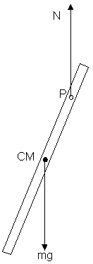
You've previously studied the simple pendulum, which is composed of a compact mass suspended from a thin cord. (See L105.) The mass of the cord is assumed to be much smaller than the mass of the bob, and the dimensions of the bob are assumed to be much smaller than the length of the cord. Ideally, one has a point mass suspended from a massless cord. If the pendulum is allowed to swing with small amplitude oscillations, the period of oscillation is given by T = 2π(L/g)^0.5, where L is the length of the cord. In this lab, we study a physical pendulum. For the latter, there is no requirement that the oscillating mass be compact. The physical pendulum can be an object of arbitrary shape rotating about an axis either within or outside of the object. Figure 1 represents a generalized physical pendulum. The period of oscillation of a physical pendulum is given by T = 2π[I/(mgr)]^0.5, where I is the moment of inertia of the object about the axis of rotation, m, is the mass of the object, and r is the perpendicular distance from the axis of rotation to the center of mass of the object. This formula is given without proof, and the student is not required to know how to prove it. However, one should know the assumptions for which the formula is valid. These are the following:

1. Frictional forces are negligible.
2. The amplitude of oscillations is small (less than 10^o from the vertical).

Now we'll look at the dynamics of the motion of a physical pendulum. Refer to Figure 2 to the right. The pendulum will be a stick of rectangular cross section and uniform density suspended from a pin at point P about which the stick can swing freely. The two forces acting on the stick are shown. These are the normal force, N, acting at the pivot pin and the weight of the stick, mg, acting from the center of mass of the stick, CM. These forces are in equilibrium.

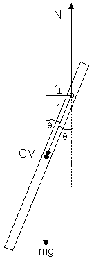
Now refer to Figure 3 to examine the torques on the stick. If the pivot pin is taken as the axis of rotation, then the normal force contributes 0 torque, since that force passes through the axis of rotation. The weight of the stick, on the other hand, will contribute to the net torque. Let r represent the position vector of the CM. r extends from the axis of rotation to the CM. With θ representing the angle between the vertical and r, the moment arm of mg is . Thus, the magnitude of the torque exerted by the weight about the axis of rotation is |τ_mg| = mgrsinθ.

Using the second law for torque, we have τ_net = Iα, where α is the angular acceleration of the stick. Substituting torques produced by the forces, we have τ_net = τ_N + τ_mg = 0 + τ_mg = τ_mg . Substituting the expression for τ_mg above and solving for α, we have the following: |α| = mgrsinθ/I. Note that we place the angular acceleration in absolute value marks to indicate that we're only interested in the magnitude of the angular acceleration. As the stick oscillates, the angular acceleration will change signs at the extremes of the cycle.

We next need to solve for the moment of inertia of the stick in terms of the mass, m, and length, L, of the stick as well as the distance, r, between the axis of rotation and the CM. From Table 10-1 of the text, we find that I_CM = mL²/12. Note that this is the moment of inertia about the CM. In order to obtain the moment of inertia about the axis of rotation, we use what's called the parallel axis theorem. This tells us that if we translate the axis of rotation parallel to itself from the CM of an object a perpendicular distance, x, away, then the moment of inertia about the new axis is I_x = I_CM + mx². Thus, the moment of inertia of the stick about the axis of rotation is I_r = mL²/12 + mr². We substitute this expression into that for the angular acceleration to obtain the following.

|α| = mgrsinθ/(mL²/12 + mr²) = grsinθ/(L²/12 + r²)

Since the angular acceleration depends on θ, we can't solve this equation using the formulas for objects rotating with constant angular acceleration. The method of solution will have to be left for a physics with calculus class.

The method of the experiment will be to measure the period of oscillation of a stick as a function of the distance of the axis of rotation from the center of mass of the stick. The experimental result will then be compared to the theoretical equation: T = 2π[I_r /(mgr)]^0.5.

 Equipment

Use these items from your lab equipment:

• Meter stick (actually, it's been cut off so it's less than 1 meter)
• Large paper clip (originally taped to the meter stick when it was shipped to you)
• LabQuest Mini interface with USB cable
• Photogate with cable

You provide these items:

• Support for the pendulum (could be a table or your desk top)
• Books (for support and risers)
• Tape (such as blue tape)
• Computer for connection to LabQuest

 Design

• Examine the sawed-off meter stick. It's actually about 36 inches long, so you could call it a yard stick if you prefer. We'll just call it the stick from this point on. You'll see small holes drilled at intervals along the length of the stick. These will serve as pivot points. If you straighten the paper clip and insert it through a hole, you can suspend the stick from the clip and set the stick into oscillation as a physical pendulum. Thus, you can see how you'll easily be able to change the distance between the CM and the axis of rotation. When you measure the positions of the holes, measure to the nearest millimeter.

• You'll need to determine where the CM of the stick is. Don't assume it's at the geometric center, because the wood may not be of uniform composition. You'll need an operational method to determine where the CM is. You could, for example, balance the stick on a credit card or a knife blade. As part of the prelab, you'll determine the position of the CM.

• You'll need to set up a steady support for the stick. You could, for example, tape the paper clip near the edge of the table so that the wire extends over the edge. Then stack books or other weights on the clip to hold it steady.

• Remind yourself how you set up the photogate to measure time in L131. For that experiment, you set the photogate on the floor and used it to measure the time for the pendulum bob to pass through the gate. In this experiment, the photogate will be positioned similarly. However, you'll need some way to adjust the vertical height of the photogate, since the length of the stick below the support will change whenever you change the point of support. You could just have a big stack of books handy to use as risers. The good thing is that alignment of the photogate isn't critical as it was in L131. All that's important is that the photogate be held motionless for each measurement of period and that the stick swings freely through the gate.

• The timing program that will be used in Logger Pro is called Pendulum Timer. It works like this: The first time the stick passes through on its downward swing, timing starts. The second time the stick passes through, nothing happens. The third time, timing stops. Think about it and you'll realize this will give a measurement of 1 period. Also, the width of the stick doesn't matter, because it's the same leading edge of the stick that starts and stops timing.

• You'll be measuring time intervals of seconds rather than the very short intervals you measure in L131. This should enhance accuracy so that it's not necessary to take as many time trials as in the past. Three trials for each value of the independent variable should be sufficient.

 Method and Data

Print this page for your original data.

1. You've already measured the length of the stick, the position of the center of mass, and the positions of the axis holes. Enter the same values on your original data page, unless the teacher has indicated that you need to make corrections.
2. The first axis hole is very near the 0 end of the stick. If this hole is unusable, then start with the next hole around the 5 cm mark. Suspend the meter stick from a sturdy support and set up the photogate as described in the Design section.
3. Connect the photogate to DIG1 on the LabQuest, and connect the LabQuest to the computer. Open this experiment in Logger Pro:

on a Mac: File -> Open -> Applications -> Logger Pro 3 -> Experiments -> Probes & Sensors -> Photogates ->Pendulum Timer.cmbl

on a Windows computer: File -> Open -> Program Files -> Logger Pro 3 -> Experiments -> Probes & Sensors -> Photogates ->Pendulum Timer.cmbl

Once the experiment opens, go to Experiment -> Data Collection and set the Duration to 2000s. This will allow Logger Pro to continuously take data throughout the experimen (or about half an hour).

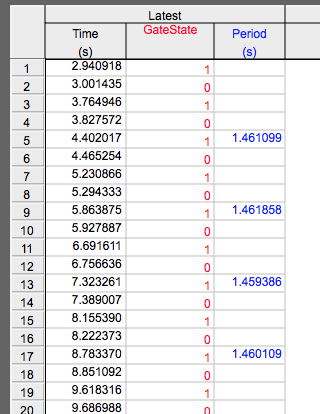
4. Keep the amplitude of oscillations of the stick small. Start with the stick far enough to the side so that it clears the photogate and is completely free of your fingers before it first enters the photogate. If the stick has much wobble (twist) as it oscillates, try releasing it in such a way as to reduce wobble. Holding the stick with a finger on each side and opening both fingers quickly is a good method. As mentioned in the Design section, timing starts the first time the stick enters the photogate and stops the third time the stick enters. (This doesn't mean that you should stop the timing yourself. The program will automatically generate the data for the Period column of the data table as the stick swings. See the screen capture from a typical experiment to the right.)

Take at least three measurements of period for each axis position. Once you start timing with Logger Pro by clicking the go , don't stop timing--that is, don't click the stop button, until you've completed all trials for all axis positions. Each successive period will simply be added to the table in Logger Pro. This way, you'll have all the times in a single file in case they're needed for reference later. When you have all your times, save the file with the name, L143D-lastnamefirstinitial.cmbl. You'll submit this file with your original data page.

5. Move the point of support to the next hole on the stick, and adjust the position of the photogate accordingly. Take 3 more time trials. Continue this process, moving the point of support about 5 cm closer to the CM each time, adjusting the photogate, and taking 3 time trials. The last point of support should be at the hole that is about 5 cm from the CM. Avoid using the hole nearest the CM, as the period of oscillation approaches infinity as you approach the CM.

Scan your original data, name the file L143D-lastnamefirstinitial.pdf, and submit it to WebAssign L143D along with the LP file.

 Analysis

You'll use Logger Pro for analysis. However, you won't do a curve fit this time, since the theoretical formula for period isn't a simple relationship. Do the following to prepare, enter, and plot your data and compare to theory.

1. Download this calculator spreadsheet to calculate % mean deviations and check your values of (x_cm - x_ax). Save the file with the name L143C-lastnamefirstinitial.xls.
2. Open a new file in Logger Pro and save it with the name L143-lastnamefirstinitial.cmbl. Change the X column in the data table to a column for the values of r = (x_cm - x_ax) and copy the values from your spreadsheet.
3. Change the Y column in the data table to one named T_exp and copy the values of mean periods from your spreadsheet.
4. Create a manual column for the % mean deviations in period.
5. Develop a theoretical formula for the period of the stick in terms of r, L, and g. (See the theory section.) Next create a calculated column that you name T_thy. Before entering the formula in the Expression window, click on the Parameters drop-down box and select Edit Parameters. Then create a parameter for the length L of the stick and another for the value of g. Click OK. Now enter the theoretical formula for the period in terms of the variable r and the defined parameters. Note that there's already a definition for pi.
6. You should now have a column of measured periods and theoretical periods. Plot a graph of period vs. r, where you plot both T_exp and T_thy on the vertical axis. In order to get two variables to appear, click on the y-axis label and select More. Then select the variables to plot.
7. Two data series should now be displayed on your graph. If you entered your formula for T_thy correctly, then the experimental and theoretical points should be very close together. That's to be expected for this experiment, because the periods can be measured very accurately, and the theory is very good. Before moving on, set the error bars on T_exp using the %MD column. Remember to set this as a percentage.
8. Create a column for the residuals, namely, the differences T_exp - T_thy. Insert a new graph to plot the residuals.
9. Check that your graphs are descriptively named, all variables have SI units, and the Displayed Precision is appropriate for values in the data table.

  Error Analysis

Answer the following in a text box.

1. Do the error bars (% mean deviations) account for any differences between theory and experiment? Describe and explain.
2. A hundredth of a second or less is considered small for the residuals. Are all of your residuals small? If not, which ones exceed the smallness criterion?
3. You may find that the residuals are consistently either positive or negative. This is a common result in this experiment and is indicative of systematic error. Describe two possible sources of systematic error in the experiment. Make it clear in your descriptions why the errors would make the residuals either consistently positive or negative.
4. Kinetic friction of the meter stick rubbing against the paper clip inside the hole is an external force that may contribute to error in the experiment. In order to contribute to error, though, the friction would need to produce a torque. You might think that there's no torque due to friction, since friction acts at the axis of rotation. That's not quite correct, though. What is the moment arm of the friction force (approximately)?
5. Describe two other possible sources error that weren't addressed in items 3 and 4 above.

 Conclusion and Submission

Write a conclusion summarizing what you did and what you found out. Then submit your Excel and LP files to WA L143.

© North Carolina School of Science and Mathematics, All Rights Reserved. These materials may not be reproduced without permission of NCSSM.