Goals

Use the known relationship between the velocity of a pendulum bob at its lowest point and the vertical distance of fall of the bob to determine the value of g.

 Prelab

Part A. Read the Introduction below. Then complete L131A on WebAssign.

Part B. Equipment set up

1. Examine the Equipment List and view the video under Equipment Setup below.

2. Set up your experiment so that it's ready for taking measurements. Take a photo of your set up being sure to show all parts, including the experimenter (you!) ready to release the ball. You could have a parent, sibling, or friend snap the photo. Submit your photo to WebAssign, L131B.

 Introduction

Theory

An ideal, simple pendulum consists of a point mass suspended from a massless string. The bob swings in a circular arc under the influence of gravity. In the real world, the string has mass and the bob isn't a point. However, it's easy to approach the ideal by using a lightweight string, and a small, dense bob. In this context, small means that the size of the bob is small compared to the length of the string. Dense means that the bob has a large mass to volume ratio similar to that of, say, a metal or even wood. (A wad of paper wouldn't be a good choice.) With choices such as these and a firm support for the string, the pendulum becomes a good device for studying conservation of energy, because non-conservative forces such as air friction and friction in the support do not play a large part over the course of a cycle of the motion.

We'll begin by analyzing the motion of the pendulum in terms of forces and will then tell why conservation of energy is a better method to use for this situation.

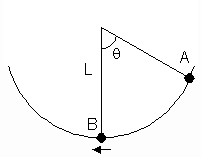
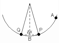
The situation is shown in Figure 1 below. The string of length L is pulled to an angle of θ with the vertical and released from rest at point A. The goal is to determine the speed of the bob at point B. The acceleration of the bob isn't constant, so one can't, in principle, use dvat equations. Let's see why.

Figure 1	Figure 2	Figure 3

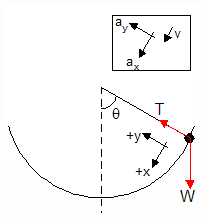
In Figure 2, we've drawn the forces acting on the bob when in position A. Tension acts toward the center of the circle and weight acts vertically downward. Unlike previous problems we've had, there are two acceleration components. There's a component toward the center of the circle, but there's also a component tangent to the circular path. This latter component causes the bob to speed up if it's headed down or causes the bob to slow down if it's headed up.

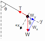
In order to write net force equations, we select axes parallel and perpendicular to the bob's velocity vector. In Figure 3, we've resolved the weight force into components along the axes. The net force equations are the following.

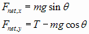
Applying Newton's 2nd law to the F_net,x equation yields a_x.

This shows that the acceleration of the bob tangent to the path is non-uniform. The acceleration depends on the angle θ, which is changing. This is the reason we can't apply dvat equations to the solution of the problem of finding the speed of the bob at the lowest point. The dvat equations assume uniform acceleration.

This leaves conservation of energy as the method of choice for the problem. For conservative forces, of which gravity is one, we need know only the initial (A) and final (B) states of the pendulum. We don't need to know the path followed by the bob, because the work done by gravity is independent of the path, and the work done by tension is 0. You'll solve the conservation of energy problem as part of the prelab.

Experiment

Let's revisit the situation with the series of diagrams below. Figure 4 is the same as the previous Figure 1. Figure 5 adds horizontal line AC in order to define the distance CB that the bob falls vertically from points A to B.

Figure 4	Figure 5	Figure 6

From the application of conservation of energy to the system of the pendulum and the Earth, the speed of the bob at point B is the following. Note that (y_A - y_B) = CB.

v_B = [2g(y_A - y_B)]^0.5

Measuring the magnitude of the maximum velocity

Theoretically, you need to find the instantaneous velocity at the bottom of the swing. In practice, you'll have to settle for an approximation. Consider Figure 6 above. If you measured the time, Δt, for the bob to travel from P to Q (equally-spaced on either side of the vertical), then an approximation to the speed at the lowest point would be:  v_ave = Δx/Δt, where Δx is the straight-line distance from P to Q. The closer together P and Q are, the better your approximation would be, in principle. We have to add the phrase, in principle,  because in practice the uncertainty increases as the time interval decreases. Suppose, for example, that Δt is 0.4 s with an uncertainty of 0.1 s in starting and stopping a stopwatch. That's a 25% uncertainty. If a smaller Δx is used so that Δt is, say, 0.2 s, then the percentage uncertainty increases to 50%. So there are two things working against each other here. Theoretically, v_ave approaches the instantaneous velocity, v_B, as Δx decreases; however, experimentally, the measurement becomes highly uncertain. Here is the approach we use to deal with it.

We use a photogate to minimize starting and stopping error. The photogate is placed at the bottom of the pendulum's swing. The photogate starts a timer when the bob enters it and stops the timer when the bob leaves. With this method, timing uncertainties can be reduced to thousandths of a second. Moreover, the distance Δx over which the timing occurs is limited to the width of the bob. Accurate results can be expected with this method. Here are some tips for getting good results:  a) Make sure the photogate is positioned at the lowest point of the swing, b) Make sure you know which points of the bob are triggering the photogate on and off. You have to know this, because that gives you your distance, Δx. If the bob were a cube, then Δx would depend on how the cube is turned as it passes through the gate. Therefore, a cube is not a good choice for the bob. A sphere is a better choice, since it doesn't matter if the sphere rotates as it passes through the gate. However, it's important to position the sphere vertically so that the photogate beam has the same elevation as the center of the sphere. That way, you can say that the distance Δx is the diameter of the sphere.

Measuring the vertical distance of fall

One method of measuring the vertical distance of fall is simply to prop a meter stick up vertically from the floor. Measure the distance from the floor to one point of the bob, say the bottom, and measure the distance from the floor to the same point of the bob when it's in position A. The absolute value of the difference of the two positions gives y_A - y_B.

Another method is to measure the angle θ shown in Figure 2. If L is the distance from the point of support D to the center of the bob, then the line segment CB, which equals (y_A - y_B), is also equal to L(1 - cosθ).

Measuring vertical distances directly using a meter stick is the more accurate of the two methods. It's much more difficult to get a good angle measurement than to measure two vertical distances from the floor. Here's why. With the protractor, you have to make alignments with both the vertical and with the string. It's very easy to make an error of a degree or two with either of these measurements. That may not sound like much but consider how the vertical position of the bob at point A would change if the angle of the string were changed by a few degrees. With a string length of half a meter, a deviation of a few degrees could change the vertical position by 1 to 2 cm. Again, that may not seem like much. If, however, the distance of fall is, say, 10 cm, that's a 10 to 20% error.

 Equipment List

From your lab kit

• white, nylon string
• steel ball
• LabQuest Mini interface and USB cable
• photogate and cable to connect to interface

You provide

• meter stick
• computer for data collection
• tape to hold items of equipment in position
• a table or chair to suspend the pendulum from

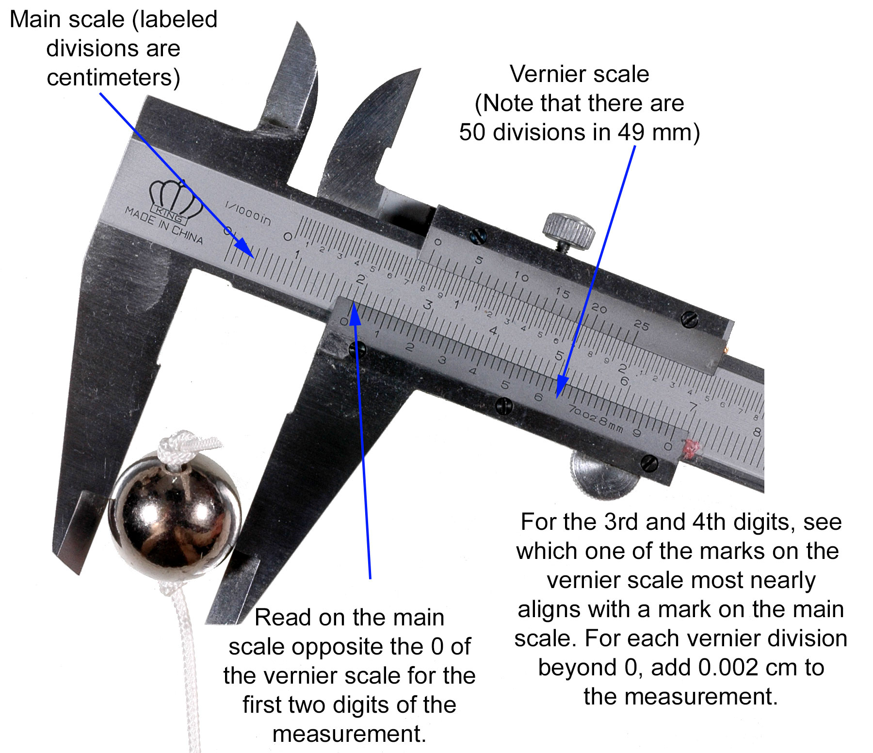
The teacher will provide a vernier calipers (for measuring the diameter of the ball).

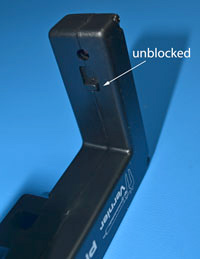
Important note about the photogate: There's a slider on the inside surface of one of the posts. Make sure this slider is in the unblocked position. See the photo to the right.

 Equipment Setup and Design

Download and watch this QuickTime movie to see how to set up the experiment. Then set up your own equipment.

Setup

Here is a list of important points about the experimental set up that will help you in obtaining good data. These points are also mentioned in the video.

1. Tie the bob between half knots at the end of the string to make sure the bob can't slip along the string.
2. Anchor the string securely with tape at the top. If the string slips, then the alignment of the bob with the photogate will change.
3. Align the bob with the photogate beam. First locate the two holes in the photogate between which the infrared beam passes. Then make sure that the bob is centered on the beam when the string hangs vertically. Orient the photogate so that the beam is perpendicular to the plane of the pendulum's swing.
4. Use the meter stick in vertical orientation to measure heights. Know where your zero level is and make all height measurements from that zero level.

Design

The variables

The setup is part of the design, but there's more to the design than just the setup. The design has to do with selecting the independent and dependent variables and deciding how to determine the relationship between them. From past experiments you had experience in determining a relationship following these steps:

1. measuring the dependent variable as a function of the independent variable,
2. plotting the data,
3. re-expressing a variable if needed to obtain a linear relationship,
4. performing a fit,
5. using a matching table to compare the fit to the theory.

In this experiment, the independent variable is the height (y_A - y_B) through which the bob falls, and the dependent variable is the speed, v_B, of the bob at the bottom of the swing. Since a linear relationship is not expected, the process of fitting the data will require a re-expression of one of the variables. This will be discussed further down.

Selecting values of the independent variable

In order to get a smooth curve that will provide a good fit to the data, you need to have a sufficient number of values of the independent variable. At the lower limit, you won't get a curve from less than three values, but three values aren't sufficient for a good fit. Ten values would be fine, but you have to consider how much time you have to collect data. Five or six values is a typical compromise. Having made that decision, then you have to consider how to spread values of the independent variable over the domain. The domain, in this case, would be distances of fall from a little more than 0 to the length of the string (The latter would be a 90° angle of release.). For a quadratic relationship, you'll need to space values closer together near the 0 end of the domain and then spread them further and further apart as you approach the maximum. The reason for this is that the function changes fastest near the origin. An example of a spread of values of the distance of fall would be 2, 5, 10, 20, 35, 65 cm. Of course, you shouldn't try to replicate these values exactly. Note that the highest value in the series is about the distance that would be available under a typical desk.

Testing for reproducibility

Take five trials for each value of the independent variable in order to evaluate the reproducibility of the measurement.

 Data

Having set up and designed the experiment, you're ready to take data. Download and print this pdf of a table to record your original data. Record in pen as usual for original data. You'll submit your original data in advance of the report due date.

Distance measurements

1. Note the units of measurement in the table. Be sure to record values in these units.
2. Measuring distances on the meter stick to the nearest millimeter is the best that can be expected, considering the uncertainties inherent in sighting measurements.
3. When you read heights on the meter stick, move your head so that your line of sight is perpendicular to the stick.
4. Read and record the height of the bob with the pendulum string in the vertical position. This is y_B. Be consistent in what part of the ball that you measure from. It doesn't matter whether it's the top, bottom or center as long as it's always the same point. Pick something convenient.
5. Click on the photo to the right to measure the diameter of the ball to the nearest 0.0001 m. If you need to review how to read vernier calipers, see this animation.

Time measurements

1. Connect the LabQuest to your computer and the photogate to Dig 1 if you haven't already.
2. Open Logger Pro. From the Logger Pro menu, make the following selection. Note that the path may a bit different than the one shown. The important thing is to navigate to the Experiments subfolder of the folder where the Logger Pro software is installed on your computer.

• on a Mac: File -> Open -> Applications -> Logger Pro 3 -> Experiments -> Probes & Sensors -> Photogates ->One Gate Timer.cmbl
• on a Windows computer: File -> Open -> Program Files -> Logger Pro 3 -> Experiments -> Probes & Sensors -> Photogates ->One Gate Timer.cmbl

The only thing you'll pay attention to is the Gate Time. Ignore everything else. The Gate Time gives the amount of time that the photogate is blocked. Click the Go button and pass your hand through the photogate to register a Gate Time. Then stop data collection. The times should be displayed to 6 decimal digits. If they're not, double-click on the Gate Time column heading, click on the Options tab, and change the Displayed Precision to 6 decimal digits.

3. Save the file now with the name L131data-lastnamefirstinitial.cmbl. As you take data, save the file frequently in case Logger Pro crashes or you accidentally erase something and need to retrieve the file.
4. Get ready for your first measurement of the gate time. Position the meter stick where you want it and pull the bob over to the stick. Keep the stick vertical and the string taut. Read the position of the ball on the meter stick. This is y_B. Remember to have a line of sight perpendicular to the stick and read from the same point of the ball as you did for y_B.
5. Click the Go button to start data collection. Release the bob quickly by separating your fingers. If you let the bob slip through your fingers, you'll introduce an external force of friction. Catch the bob as soon as it passes through the photogate. Then bring the bob around the gate and back to the stick for the next trial. Don't stop data collection. You can do one release after the other this way right through to the end of the experiment. Don't stop and erase runs along the way. As you take each trial, record the time to 6 decimal digits in your handwritten data table before taking the next trial.
6. Save the Logger Pro file frequently as you take data. You'll probably have trash values in the data table from times when you accidentally let the ball pass through the gate when you weren't ready. That doesn't matter as long as you have all the good data in the file. Now how do you know when a reading should be trashed? Here are some possibilities: i) you didn't catch the ball to keep it from swinging back through the gate, ii) you accidentally let go of the ball before you were ready, iii) the ball hit the photogate. If there's an obvious reason why the data is bad, don't write the value in your data table. (Of course, it will still be in the Logger Pro file.) Here's a reason not to trash data: If, when compared to other trials, the reading seems to be further off than you would like. DO NOT DELETE DATA on the basis of a suspicion that it may not be good.
7. When you have all the data, save the file one last time.

At this point, submit the Logger Pro file and a scan of your original data page to the WebAssign assignment, L131D.

 Calculations

Now that you've collected your data, you're ready to do the calculations. In order to streamline this process, download this Excel spreadsheet which does the calculations automatically as you enter the data from your original data table. Read the instructions on the spreadsheet carefully. These are in the orange cells. It's your responsibility to check the calculated results to make sure that you're using the spreadsheet correctly and that it's calculating correctly. We recommend doing all the calculations for one of the release heights with a hand calculator as a check.

Rename the file L131C-lastnamefirstinitial.xls for submission with the rest of your report, which will be a Logger Pro analysis file.

 Analysis

You'll do the analysis in Logger Pro. Since a non-linear relationship is expected, you'll need to re-express the independent variable in order to linearize the relationship. Now here's what to do.

1. Create columns in your Logger Pro data table for (y_A - y_B) and v_B and enter the calculated values from your Excel table. This will be 5 or 6 pairs of values.
2. Plot a graph but don't fit it. You should see an obvious non-linear relationship. If Logger Pro connected the data points with lines and without point protectors, you should know by now what you need to do to change that.
3. Now you'll add horizontal error bars to your data points. Let's consider the uncertainties in the height measurements. Determing the distance fallen requires two height measurements in which you sight across to the meter stick. Estimate for yourself the absolute uncertainties in the two measurements. Find the sum of the uncertainties in units of meters. You'll use this for your horizontal error bars. Add the error bars as follows: i) Double click on the header of the (y_A - y_B) column of the data table. In the Manual Column Options window, click on the Options tab. Make sure Error Bar Calculations, Fixed Value, and Error Constant +/- are checked. For the Error Constant, enter the absolute uncertainty that you calculated for the (y_A - y_B) measurements. Click Done. You should see that the error bars have been added to the graph. If they're small, you may find them difficult to see.
4. For vertical error bars, you'll used the % Mean Deviation. First, create a new, manual column in the data table by selecting Data -> New Manual Column. Use this column to enter the values of %Mean Deviation in v_B. Enter the values from your Excel table. Next, double click on the v_B column header to bring up the Manual Column Options window. This time, select Percentage under Error Bar Calculations. For Use Column, select the %Mean Deviation column. When you click Done, a box will appear basically asking if you know what you're doing. Select Yes. Now you have both horizontal and vertical error bars on your graph. You can think of these as a visual display of the region of uncertainty surrounding each data point.
5. Re-express the independent variable as needed to linearize the relationship. Then make a new graph using the re-expressed variable.
6. Fit a straight line to the new graph. The error bars for v_B will carry over to the next graph. The size of the error bars relative to those for (y_A - y_B) depend on the re-expression. Generally the process of taking a variable to the nth power multiples the uncertainty by |n|. This applies to both integer and fractional values of n.
7. Create a graph for the residuals of the fit. This will require creating a column for the values of v_B calculated using the fit equation. Call this v_B fit. Then create a calculated column for the difference of v_B fit and v_B. Plot the residuals. If you need to review the process of creating residuals, see your L113 analysis.

Do the following in a text box in a Logger Pro.

8. Write your matching table and equation of fit.
9. Use the slope of the fit to calculate an experimental value for g. Then find the experimental error.
10. Based on the graph of the residuals, evaluate the goodness of the fit. Review L113 as needed for the two features of the residuals graph that you must discuss.
11. Another test of the goodness of fit is whether the line of fit passes through the region of uncertainty--as determined by the error bars--surrounding the data points. Describe the results of this test of goodness of fit for your data.

 Conclusion

In the text box, write a conclusion in which you describe the method of the experiment and the analysis and present your results.

 Submission

Submit your Excel table and your Logger Pro analysis file to WebAssign assignment L131.

© North Carolina School of Science and Mathematics, All Rights Reserved. These materials may not be reproduced without permission of NCSSM.