You'll do a video analysis in Logger Pro to study the motions of dropped and projected marbles. |
Prelab
You'll have time during the next WebEx session to work on the analysis. Prepare for the session by doing the following.
- Read through the Introduction of the lab.
- Download and play the following video clip: projectile-drop-3.mov. If you can't play the clip, you probably don't have QuickTime installed or working on your computer. Go to the Software page for information about downloading and installing QuickTime. (If you have a Windows platform and Windows Media Player attempts to play the movie, click here for a remedy.)
- Complete through the section Marking the Video Clip. If Logger Pro will not play the movie, then you may be using an outdated version of Logger Pro. Make sure you're using the latest version, as given on the Software page.
- Save your file with the name L113-lastnamefirstinitial.cmbl. Upload it to WebAssign L113PL before the WebEx session.
Goal
Investigate quantitatively the horizontal and vertical motions of a dropped and a projected marble.
Plan
During the WebEx session, you'll do the following:
- Prepare graphs of horizontal and vertical position as a function of time.
- Scale the time axis to match the actual conditions under which the video was obtained.
- Fit x vs t and y vs t graphs to the appropriate functions.
- Interpret the results.
You can ask questions of the teacher during the session.
Introduction
In the absence of air friction and any forces other than gravity, objects fall with the same acceleration independent of their mass. This applies as long as they are in the same gravitational field. This means, for example, that they are the same distance from the center of the Earth. This stipulation is necessary, because the acceleration of a falling object depends on the value of the gravitational field. That value at the surface of the Earth is 9.8 N/kg. The hundredths digit shows variation depending on the location on the surface of the Earth. In North Carolina, the value is 9.80 N/kg to 3 significant figures.
If we can arrange to set up an experiment where two objects are released from the same height at the same time with 0 vertical velocity, then at all times during their fall--in the absence of friction--they should have the same vertical position. This will be true even if one of the objects has horizontal motion, since the vertical and horizontal motions are independent. The video clip that you downloaded shows two marbles released under those conditions. In this lab, you'll measure the positions of the marbles as a function of time, plot graphs of their horizontal and vertical motions vs. time, and determine acceleration and velocity from the graphs.
Here's how the video was created, The red marble was initially resting on the tip of magnetically-controlled plunger. The white marble rolled down a ramp which isn't shown, and left the ramp moving horizontally. At as nearly this instant as technically possible to engineer, the plunger under the red marble was retracted, allowing it to fall. The white marble passed slightly in front of the red marble; there was no contact between them. The video itself was originally a single still image. The marbles were illuminated by a series of 12 flashes of light 0.0250 s apart, and the camera shutter was open the entire time the marbles were falling. This one image was later decomposed digitially into a series of 12 frames, each frame showing only a single pair of images of the marbles. This allows the motion to be analyzed using video analysis software.
Marking the Video Clip
You'll do everything in Logger Pro. Since this is your first time to do video analysis in Logger Pro, we'll lead you through it. For reference, here are the common functions associated with Logger Pro analysis.
-
Open Logger Pro. On the menu, select Insert -> Movie and navigate to the movie projectile-drop-3.mov that you downloaded for the prelab. Click OK. The first frame of the video clip should appear inside a window. When the movie appears, drag the corners so that it fills the available space as much as possible. This will enable greater accuracy in point placement.
-
 The
motion controls are in the lower left of the movie window. View the movie by pushing the play button. Rewind the movie by dragging the slider at the
bottom of the window all the way back to the left. Also try using the
forward and backward step buttons to view the video frame-by-frame. Step the video to the frame with the meter stick.
The
motion controls are in the lower left of the movie window. View the movie by pushing the play button. Rewind the movie by dragging the slider at the
bottom of the window all the way back to the left. Also try using the
forward and backward step buttons to view the video frame-by-frame. Step the video to the frame with the meter stick. -
Click on this button,
 , at the
lower left of the movie window. This will open a column of icons on the
right side of the move window.
You'll scale the video to the real world next. Click on this icon:
, at the
lower left of the movie window. This will open a column of icons on the
right side of the move window.
You'll scale the video to the real world next. Click on this icon:  . Then, on the video frame, click
and drag from the 30 to the 60 cm marks on the meter stick. Release the mouse and
then type in the actual distance. Note units.
. Then, on the video frame, click
and drag from the 30 to the 60 cm marks on the meter stick. Release the mouse and
then type in the actual distance. Note units. -
Next place the coordinate axes. Click on this icon:
 . Now click on the bottom of the 2nd image of the white marble. This is the first image in which the marble is completely clear of the dropping apparatus. When you release the mouse, the yellow axes will appear. You can click and drag these if you wish. Of course, the placement of the axes is simply a convenience. You can place them anywhere.
 -
Now you'll analyze the video clip by marking the positions of the marbles in each frame of the video. Step the movie to the frame where the red and white marbles seem to overlap. This is the 3rd frame after the title frame of the movie. Click on this icon,
 , to begin
marking points. Now position the cross hair cursor carefully
at the bottom of the white marble and click once to mark that position. (The bottommost point is picked because it's easier to locate than, say, the center of the marble.) A
solid dot should appear. Data will automatically be added to the data table,
and a point will be plotted on the graph. Ignore the data
table and graph at this point in the process.
, to begin
marking points. Now position the cross hair cursor carefully
at the bottom of the white marble and click once to mark that position. (The bottommost point is picked because it's easier to locate than, say, the center of the marble.) A
solid dot should appear. Data will automatically be added to the data table,
and a point will be plotted on the graph. Ignore the data
table and graph at this point in the process. -
The movie will automatically advance to the next frame. Mark the position of the white marble again (ignore the red marble for now). Continue this process to the last frame.
-
Save your file so that if you have a program crash, you don't have to mark all those points again. Save your file frequently hereafter.
-
Back up the video to the frame where you marked the first position of the white marble. Next you'll mark the positions of the red marble. Click this icon,
 , and
select Add Point Series. Click again. Now
you'll mark points for the red marble. This point series will have a
different color than that for the white marble. Go ahead and mark all the
points for the red marble.
, and
select Add Point Series. Click again. Now
you'll mark points for the red marble. This point series will have a
different color than that for the white marble. Go ahead and mark all the
points for the red marble. -
The default time scale assumed by Logger Pro is that of a typical 30 frames per second movie (actually 29.97 fps). However, the projectile movie has a frame rate of 40.0 fps. Here's how to change the frame rate to that value. In the main menu, click on Options -> Movie Options. Click Overide frame rate and change the number to 40.0. Click OK, and you'll see all the times in your data table adjust to the new value. Note that the first time is 0.075 s, corresponding to the 3rd frame from the title frame. In the event that Movie Options is grayed out on your computer, here is an alternative way to change the time scale:
- Select Data -> New Manual Column from the menu.
- Enter an appropriate name such as Time-act (for actual time) and units of s.
- Select Generate Values.
- For Start, enter 0, and for Increment, enter 0.025. For End, multiply 0.025 by (number of data points - 1). Click Done to generate the column.
- On your graph, click on the Time label on the horizontal axis and select your new time variable.
- Finally, delete the original Time column in your data table.
-
When you're finished marking points, you'll have a data table and a graph of horizontal (X) and vertical (Y) positions vs. time.
Formatting the Data Table
Take some time now to rename the variables and eliminate some columns from the data table to avoid confusion. Do the following.
-
Delete the two Vx and two Vy columns from the data table. Those columns will not be helpful. From the main menu, select Data -> Delete Column. Then select the column you want to delete. You have to do this one column at a time. (Note that is not the same thing as deleting original data, because the velocity columns are calculated automatically using the X and Y columns, which are original data and are not deleted.)
- Change the names of the variables to Xw, Yw, Xr, and Yr using r and w to distinguish the marbles. Set the Displayed Precision for all variables to 3 decimal digits. (Recall from L105 that the way to do this is to double-click on the corresponding column heading.)
Graphical Analysis
Horizontal motion of the white marble
- By default, all variables are plotted vs. Time in the graph window. Click on the y-axis label and select More. Uncheck all the selections except for Xw. For Scaling, select Autoscale from 0. Click OK. Then double-click and set the usual properties: title, point symbols, no connecting lines. An appropriately descriptive title is Horizontal Position vs. Time for the White Marble. (At this point, we'll stop reminding you about formatting and scaling choices and simply expect you to do them.)
- You know from your study of projectile motion to expect the horizontal velocity to be constant. That should inform your choice of how to fit the data. Perform the fit.
- Insert a text box on the page and prepare the matching table for the fit you just performed. Pay particular attention to the entries in the Physics for the coefficients. Name these coefficients as a standard practice. For example, for a linear fit the b coefficient (y-intercept) would be called the initial horizontal position. An easily interpreted abbreviation such as init.hor.pos. is acceptable. For the Value (Expected) column, you won't have entries, since these are not known other than by performing the fit. (The initial horizontal position isn't the position of the first image that you marked, because that is t = 0.075 s in your table. The initial horizontal position occurs 0.075 s earlier. The specific location of this point is unimportant to the analysis. However, you should expect it to be negative. Do you know why?)
- Write the physics form of the equation of the fit under the matching table.
Vertical motion of the white marble
- Insert a new graph and change the vertical variable to Yw.
- In order to help with fitting the graph, let's make a connection between the equation of fit and the physics that you learned in Chapters 2 and 4. For uniform vertical acceleration, we expect the vertical position as a function of time to be given by the dvat for vertical motion: y = yo + voyt + ½ayt². Now recall the simple pendulum experiment where you had a non-linear relationship between period and length of the pendulum. The approach to analysis there was to re-express the length as sqrt(length) and plot a graph of period vs. sqrt(length). That gave a linear relationship for which you then performed a linear fit. While this is the method of fitting that you'll use most frequently in this course, you'll use a different method in the present lab. Since you expect a quadratic relationship between the vertical position and time, you may perform a quadratic fit. Do that now by first selecting from the main menu Analyze -> Curve Fit. Then, in the Curve Fit dialogue box, select Quadratic for the General Equation. Click the Try Fit button to generate the fit. Then click OK. The fit will appear on the graph.
- Now examine the fit. Both the math and physics forms of the equation of fit are given in the table below for comparison.
quadratic term linear term constant term Math y = +At² +Bt +C Physics yw = +½awyt² +vowyt +yow Note the use of multiple subscripts in the physics equation above for o (initial), w (white), and y (vertical). By this time in your study of physics, you should be becoming more familiar with the use of subscripts as a mathematically-sophisticated way to distinguish variables of the same type according to time (initial / final) and object (white / red). Such use indicates attention to detail in your thought processes as well as in communicating your work clearly to the reader. The order of the multiple subscripts isn't important here but should be consistent to make communication more efficient.
If the fit is a good one--and it should be in this case--we expect from an examination of the table above that A = ½awy, B = vowy, and C = yow. Prepare your matching table now. This table will have more rows than the ones you've prepared before. Here's what it looks like:
Math maps to Physics Value
(graph)Value
(expected)Units y --> var var A x var var B C
- Write the physics form of the equation of fit under the matching table.
Horizontal motion of the red marble
If you examine the path of the red marble closely, you'll see that it has a small horizontal component in the negative direction. This may have been due to a small amount of friction exerted by the plunger on the marble as the plunger pulled away down and to the left. Therefore, the drop of the red marble isn't a true vertical drop, although the presence of the horizontal velocity doesn't affect the vertical motion. Do the following analysis for the horizontal motion.
- Insert a new graph and change the vertical-axis variable to Xr. Select Autoscale from 0 as you've done before.
- Perform a linear fit.
- A matching table isn't required, since you did a similar one for the white marble. Do, however, write the equation of fit in the text box.
- Now try this exercise to demonstrate how a graph can be deceptive if you don't pay attention to the scales. First, make sure the graph of Xr vs. Time is selected. Click the autoscale icon
 below the main menu. Note how the points now seem more scattered, and the slope of the fit is steeper. Of course, nothing has really changed other than the display. The vertical scale of the graph now spans a much smaller region. This makes the data look worse than it is. Now type CTRL-Z or CMD-Z to return to the previous scaling. This scaling makes more sense in comparison to the scaling for the graph of horizontal position vs. time for the white marble.
Vertical motion of the red marble
The steps below will be abbreviated compared to previous ones. By this time, you should be learning how to carry out the various operations of graphical analysis.
- Insert a new graph and change the vertical variable to Yr.
- Perform a quadratic fit.
- A matching table isn't required, since the previous one provides experience in preparing a matching table for a quadratic fit. Do, however, write the equation of fit in the text box.
Residuals and Goodness of Fit
With the labs early in the course, we introduced you to the techniques of error analysis. Rather than drop it all on you at once, we spread the subject out over several labs. So far, you've learned about increasing accuracy in measurement (L101, L105), estimating uncertainties (L101, L103, L109), finding relative error from repeated trials (L101, L105), adding error bars to graphs (L105), calculating experimental error (L103, L105, L109, L111), and discussing sources of error qualitatively (L101, L105). The next technique of error analysis to introduce you to is the graph of residuals. This is a graph which displays--as a function of the independent variable--the difference between the value of the dependent variable calculated from the fit and the value determined by measurement. For example, for the vertical motion of the white marble, the residuals would be calculated like this:
Residual = Yw (fit) - Yw
= (At2 + Bt + C) - Yw
It's not important whether you subtract the experimental value from the fit value or vice versa. Don't take the absolute value, though, as you would for a deviation. The sign of the residual is important.
Next we describe how to use Logger Pro to plot residuals and then tell you how to interpret the resulting graph. We'll only have you do this for the vertical position of the white marble as a function of time.
- Create a new calculated column in the data table by selecting from the main menu Data -> New Calculated Column. For the name, both long and short, enter Yw-Res. The units, of course, are the units of position. For some reason, people tend to omit the units of the residuals, which is incorrect. For the Expression, use A*"Time"^2+ B*"Time" + C - "Yw", where you type in the numerical values of A, B, and C from the fit of Yw vs. Time. Don't include units here. Do type in all the digits of the coefficients without rounding in order to avoid rounding error. Do double check your numbers to correct any mistakes in transcription. A single incorrect digit will completely invalidate the residual calculations. For the variables, "Time" and "Yw", simply select from the Variables (Column) drop-down menu.
-
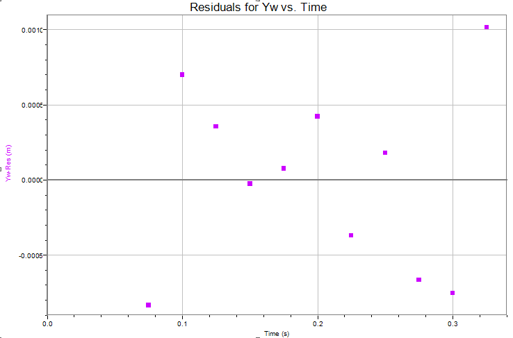
Insert a new graph. This will probably be Yw-Res vs. Time but if it isn't, select those variables. You can keep the title simple, for example, Residuals for Yw vs.Time. For residuals, you should allow Logger Pro to autoscale, because you want to see fine detail. If you need to autoscale, just click the
at the top. -
A typical graph is shown below. Compare it to yours. You should see points scattered on either side of Yw-Res = 0. If this is not the case, you may have entered a fit coefficient incorrectly. Double-click on the Yw-Res column heading in the data table to check the expression. Note the scaling of the vertical axis. It's typical for the values of the residuals to vary by no more than a few millimeters on either side of 0. There are two tests of a good fit using the residuals graph:
- The values of the residuals are small in comparison to what was measured (Yw, in this case).
- The points are randomly scattered on either side of the horizontal axis.
If either condition above is not met, the fit is not a good one. For example, if the residuals are small but there's a distinct pattern, then the fit is questionable. The example residuals below indicate that the fit is a good one.
Finding residuals is the method that we'll use in this course to evaluate the goodness of fit. We will not use the RMSE coefficient that Logger Pro generates together with fit coefficients.
A comment on the validity of the assumption of no air friction: For short distances of fall (less than 1 meter) of compact objects like the marbles, air friction doesn't play a significant role and likely doesn't result in errors in timing of even a millisecond. Such errors wouldn't be measurable in this experiment. For distances of fall of several meters, the effects of air friction would begin to show up in the data. The residuals of the quadratic fit for vertical position vs. time would show an obvious pattern in that case.
Interpretation
Continue in the text box to answer the following questions to interpret your results. Number your answers as given. Your answers will serve both as interpretation and conclusion.
-
What are the horizontal velocities of the red and white marbles? Why is the horizontal velocity of the red marble negative?
-
What is the direction, up or down, of the initial vertical velocity of the white marble? Explain. (Be sure to take note of which direction is +y for your data.)
-
Use a coefficient of the appropriate fit to determine the vertical acceleration of the white marble. Show your work. Repeat for the red marble.
-
Calculate the experimental error for each of your calculated accelerations.
-
Describe a possible reason (source of error) why the values of the accelerations calculated for the red and white marbles are different.
-
Suppose you had performed a quadratic fit instead of a linear fit on the horizontal motion of the white marble. What result would you expect for the A coefficient and why?
-
Describe the goodness of your fit for the vertical motion of the white marble. (See the two tests described previously.)
Submitting your file
A conclusion is not necessary for this lab. Your file should have a single page. Auto arrange the page and save your file a final time. Then upload it to the L113 item in WebAssign by the due time.