|
This lab requires simple measuring instruments. The lab will introduce you to techniques of graphical analysis and extend your use of error analysis from L101. |
Goal
To determine the speed of sound by using the relationship between the distance traveled by sound versus the time taken to travel that distance
Introduction
Average speed is defined by the following relationship:
Average speed = (Distance traveled) ÷ (Time taken to travel that distance)
In shorthand notation, vav= Δd/Δt, where vav represents the average speed, Δd is the distance traveled, and Δt is the time to travel that distance. The Greek letter, Δ (uppercase delta), is commonly used to represent the difference of initial and final values of a quantity. Therefore, Δd means df - di, where di is the initial distance (frequently 0) and df is the final distance. Note that one always subtracts the initial value from the final value. Likewise, Δt = tf - ti. It's important to remember that average speed is the ratio of two differences.
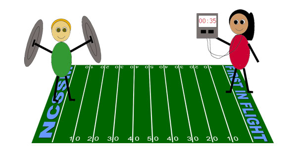
A common way to determine the average speed of an object is simply to measure how long it takes the object to travel a known distance. This is called a time-of-flight technique. Sound waves are known to travel at a speed of about 340 m/s in dry air at room temperature (20 °C). This speed is generally too fast to measure accurately by time-of-flight techniques. In one method, students stand on the goal lines at opposite ends of a football field. At one end, a student smashes two metal trash can lids together. At the other end, another student starts a stop watch when he/she sees the lids come together. (See below.) He/she then stops the watch upon hearing the sound from the lids. The time interval between sight and sound is only about a third of a second. This isn't much longer than a typical human's reaction time in starting and stopping the watch. Therefore, accurate results can't be expected with this method.
 The
method used to collect data for the present experiment is described in
the video clip Measuring the Speed of Sound, Part I. Two wooden blocks
are struck together to produce a loud sound. The sound is detected by
two microphones a distance d apart. Each microphone is connected
to an amplifier which automatically discharges a flash unit. The flashes
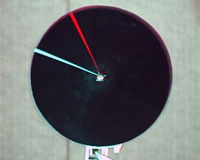
of light illuminate a disc rotating at a constant frequency. The disk,
which serves as a clock to measure the time interval between the flashes,
is black except for a white radial which serves as the hand of the clock.
The two flashes of light produce two images of the hand separated by an
angle. A typical photograph of the clock face is shown to the right.
The
method used to collect data for the present experiment is described in
the video clip Measuring the Speed of Sound, Part I. Two wooden blocks
are struck together to produce a loud sound. The sound is detected by
two microphones a distance d apart. Each microphone is connected
to an amplifier which automatically discharges a flash unit. The flashes
of light illuminate a disc rotating at a constant frequency. The disk,
which serves as a clock to measure the time interval between the flashes,
is black except for a white radial which serves as the hand of the clock.
The two flashes of light produce two images of the hand separated by an
angle. A typical photograph of the clock face is shown to the right.
Continue below to prepare for the lab.
Prelab
Do the following to get ready.
- Watch two video demonstrations so that you'll see how the data was obtained. You'll not only see the method used, but you can also get an understanding of some of the errors inherent in obtaining data. These clips last a total of about 15 minutes.Watch the videos in the order below. You'll be asked questions about the videos to answer in your lab report. Two methods are provided for viewing the clips. Streaming will work cross-platform as well as on mobile phones with no special software. The download links can be used to save the files to your hard drive. You'll need a player to view downloaded files. The VideoLan player has been recommended previously.
Measuring Frequency with a Stroboscope Stream Download Measuring the Speed of Sound Part 1 Stream
-
Do the WebAssign assessment L103PL.
-
The following guides will be discussed at the WebEx session preceeding the due date of the lab. Read these guides as preparation for your data collection and analysis.
The Lab
|
Title, Goal, Your Name, and Partner's Name
Write the Title, Goal, Your Name, and Partner's Name in the appropriate places in your report. For the goal, use the goal as stated in the prelab. You need not rephrase the goal. Since you're not working with a partner on this lab, write No Partner.
Theory
Derive the equation for the measured speed of sound vsound in terms of the frequency f of the clock, the angle A between images of the hand on the disc, the distance traveled by sound between flashes, Δd, and the number of degrees in a circle. Justify the steps in your derivation. A list of equations isn't sufficient.
Example
|
List of Apparatus
You'll need the following.
- 30-cm ruler and protractor (from your lab kit)
- Recording materials: Pen and paper
- Graph paper: For this lab, you must draw the graph by hand (no software allowed). Download this graph paper template. Print hard copy.
- Set of 4 photographs for analysis: There are two sets of 4 photographs: Photo Set 1 / Photo Set 2. Download one set or the other (your choice) and print the photos.
Method
For some labs, you'll write a complete method section. For this lab, though, you need not write a method now. Instead, you'll show your knowledge of the method in the Application section near the end of your report.
Data
In order to make sure that you collect your data well in advance of the due date of the final report, a scan of your original data page will be due in advance of the report itself. See the schedule for the due date of L103D.
-
Label a section called Data in your report. Write the first item of data: frequency of the clock, f = 50.0 Hz. Note that it's not enough to simply say frequency. You must specify frequency of something. Also give the short-hand symbol for frequency. The numerical value is given to you by the instructor, since that's what the frequency of the clock was to the nearest tenth of a hertz. Note finally that the unit of measurement is given. Always include units with numerical values of measurements. In this case, Hz is the unit of frequency and is equal to 1/s or s-1. This is equivalent to the unit rotations per second or cycles per second.
- Prepare a data table like the following. Leave plenty of room for data entries. Circle the number of the Photo set that you downloaded and printed. The Photo ID is given in the upper-left hand corner of each photo, while the distance is given in the lower left-hand corner. Note that units of measurement are given in the column headings for measured quantities. Since the units are in the heading, you don't have to write them again beside the numbers as you fill in the table. You'll fill in the Angle column as you take measurements. Later, you'll calculate the value for Elapsed Time.
| Photo set used: 1 2 | |||
| Photo ID | Distance (m) |
Angle (°) |
Elapsed Time (s) |
-
For each photo in turn, align the center of the protractor with the center of the disc in the photo. Align one of the images of the hand on the photo with the baseline of the protractor. Read the measurement of angle from the other image of the hand. Be sure to read from 0°. Figure A below shows how to align the protractor. Since the images of the hand have width, you'll need to use a consistent technique for aligning the images with the protractor. We suggest always using the same side of the hand image as shown by the arrows in Figure B.
-
Read your measurements to the nearest 0.1 degree. It's expected that whenever using a measuring instrument that is ruled in divisions, that you read to a tenth of the smallest division unless instructed otherwise. This fraction will have some uncertainty, but will nevertheless be significant. (See Chapter 1 of your text for a review of significant figures.) When you write your measurements, they will be expressed as 35.3° or 22.0° to give two examples. Note the use of the zero to the right of the decimal point in the latter example. If you judge the decimal part of the reading to be nearer 0.0 than 0.1, you must express that fact by including the zero. If you don't, then your reading is judged to be precise to only the nearest degree.
-
Measure the angles for your 4 photos. Record the angles and the corresponding distances and IDs in the table.
| Figure A | Figure B |
 |
 |
-
Using the formula from the prelab, calculate the elapsed times for the corresponding angles in your table. Enter your results--with the proper number of significant figures--in the table.
-
Scan your data page, name the file L103D-lastnamefirstinitial.pdf, and upload your file as requested.
Sample Calculation
Label this section Sample Calculation, and then show one sample calculation of the Elapsed Time in your notebook. Begin by writing the formula in symbols that you will use. Then substitute values from one row of the table. Include units. Give the final result.
Example
|
Graphical Analysis
-
Your data is complete, and it's time to draw a graph. You'll plot your graph on the graph paper that you downloaded and printed. Turn your graph paper sideways to draw a graph in landscape orientation. Draw a graph following the practices described in Drawing and Analyzing Graphs. We repeat them here for emphasis.
-
Label your axes with name and units. For this lab, place Elapsed Time (s) on the horizontal axis and Distance (m) on the vertical axis. Note that you will never write x and y as axis labels! Always use the actual names of the variables.
-
Design a decimal-based scale for each axis such that your data will stretch across as much as the available grid space as possible. By decimal-based scale, we mean a scale such as that used by a ruler. Take a look at your ruler to see what we mean. There are 10 divisions between major units of centimeters. This makes it easy to read measurements in decimals. Image how much more difficult it would be if there were, say, 7 divisions per centimeter. On your graph paper, notice that there are 5 minor divisions per major division. Thus, each minor division is two-tenths of a major division. Once you've determined a scale for your graph, place equally-spaced numbers along the scale. You need only number every couple of major divisions. Also, indicate the position of the origin.
-
Title your graph at the top with the names of the variables in this form: Distance vs. Elapsed Time for Sound. Note that the first variable given is the one on the vertical axis. This is standard scientific form. Note also that a descriptive phrase is added after the variables. In this case, the phrase is for Sound. Units of measurement aren't required in the title.
-
As you plot points on your graph, first locate their coordinates as accurately as you can. Read to fractions of a minor division. Think of the graph as an instrument of analysis and use it as such. At each data point, place a large marker. We recommend a large X. You could also use a point, but be sure to surround it with a circle so that it will be easy to locate.
- As mentioned above, your graph is a tool of analysis. Theoretically,
one would expect the variables of distance and time to have a linear
relationship, because the speed of sound is constant. In reality,
your data points may not lie in a straight line because, of course,
there are always errors inherent in measurement. Since we expect
the relationship to be linear, however, it makes sense to draw the best
straight line through the data. You do this by placing a ruler
or straightedge on the graph in such a way as to split the difference
between the data points. That is, you'll have some above the ruler
and some below so that the differences average out to about 0, to the
best of your judgment. When you carry out this process, don't force the line to pass through the origin unless the origin is one of
your data points. In this lab, the origin is not a data point.
Draw your best straight line now.
-
Consider now what information you can obtain by finding the slope of the line that you drew. You know from math that slope is defined as rise/run or Δy/Δx. Of course, we don't want to use the symbols Δy and Δx in this or any lab, because those are generic symbols. For this lab, the rise and the run correspond to Δd and Δt. Thus, by finding the slope of the graph, you are finding Δd/Δt, which we've seen before is simply the average speed. When finding the slope of your line, follow the guidelines below in order to obtain the best results. Review, if necessary, the Example Graphical Analysis Exercises.
-
You'll need two points to calculate slope. Don't select actual data points for this purpose. Instead, pick two points that are actually on the line that you drew. In addition, pick points that are far apart. This will give your result greater accuracy. In general, greater accuracy is obtained in measuring greater amounts.
-
Once you've selected the two points, read their coordinates from the axes. As always, read to a fraction of a minor unit. Write the coordinates in the usual mathematical form beside each point.
-
-
On the next page of your report, continue with the analysis. Calculate the slope using the coordinates of the 2 points that you selected. Show your work. Begin with the formula for slope that applies to this experiment: vav = (df - di) / (tf - ti). Substitute the values of the coordinates and simplify to find the speed.
- It's time to prepare the matching table for your line of best fit. Draw a table like the following.
- Complete the table as follows. We'll guide you through this process since this is your first matching table.
Click here to see an example graph. While this graph was prepared for a different experiment and a non-linear relationship was obtained, the method of drawing the graph is the same as you'll use in this experiment.
Draw your own graph now.
Now select the 2 points that you'll use to calculate slope.
Math maps to Physics Value
(graph)Value
(expected)Units y --> variable m --> x --> variable b -->
In the Physics column, we write the symbols that represent the physics quantities in the experiment that correspond to the math symbols y, m, x, and b for the equation of a line. y and x are simply the variables plotted on the axes of the graph. These are d and t. The slope of the line is vav, and the intercept is the value of distance at t = 0. Let's call this do. Now fill in the Physics column.
In the Value (graph) column, we write the values determined by reading the graph. We only have values for the slope and the intercept. These are called the coefficients of the fit. You already calculated the slope. Read the intercept from the graph. Then record the two values in the table. You don't record values for y and x (d and t), because these are variables.
In the Value (expected) column, we write the values that we expect--based on theory--for the slope and intercept. You can look up an expected value for the speed of sound in air in your textbook. Avoid searching for the value on the internet, as some sites report incorrect values.
- In the Units column, write the units of each of y, m, x, and b.
-
Now you can write the equation of your best fit line. Start with the math form, y = mx + b. Replace y and x with the physics names of the variables. Replace m and b with the values--determined from the graph--of the coefficients. Include units.
| |
Error Analysis
Label the next section of your report, Error Analysis. This will be an uncertainty analysis.You have some familiarity with that from L101. In the present lab, we'll extend the uncertainty analysis to include uncertainty calculations for quantities that involve more than one measurement. Specifically, the measurements that have uncertainty in this lab are the frequency of the clock, the distance between the microphones, and the angle between the images of the hand on the clock disc. Here is the process of determining the overall uncertainty in the calculated speed of sound. In order to keep track of everything, organize your work in a table like the one below.
-
For the distance and angle measurements, write a representative value of the measurement, including units. The frequency is done for you. For angle and distance, select the values that you measured from one of the photos. Select one with an intermediate value of distance. For the speed, just give the value that you determined from your graph.
-
The next step is to estimate the absolute uncertainty in each measurement. This has been done for the two measurements that the demonstrator made. The uncertainty in positioning each microphone is about a centimeter. This is based on the finite width of the microphone and the fact that it's not clear what part of the sensitive area actually detects the sound first. The absolute uncertainy in the frequency is partly due to the precision with which the frequency can be adjusted. More importantly, there can be some drift in the frequency of the motor. Now it's your turn to estimate the absolute uncertainty in the angle measurement. Things that can affect the uncertainty include unavoidable variability in the placement of the protractor, the thickness of the lines, and the sighting between divisions on the scale. Do the following to estimate the uncertainty.
Select the photo that corresponds to your Representative Value of Measurement. Measure the angle 5 times. For each measurement, pick the protractor off the table and then place it back down again. Record the 5 values in a table like the one below, and find the mean and the mean deviation. Take the latter to be the absolute uncertainty.
-
For the distance and angle, calculate the relative uncertainty as a percentage. Recall that: Relative uncertainty (%) = 100(Absolute uncertainty) ÷ (Representative value of measurement). Generally, the result has 1 significant figure, since absolute uncertainties typically have 1 significant figure.
-
Now you're ready to calculate the relative uncertainty in the speed. The way this is done depends on how the measurements are used in the calculation of the speed. In this case, all calculations were multiplicative; none were additive. When measurements are multiplied (or divided), the relative uncertainties are added. Thus, simply add the relative uncertainties in distance, angle, and frequency to get the relative uncertainty in the speed.
-
Once you have the relative uncertainty in the speed, you can calculate absolute uncertainty using the same formula as in part c, but rearranged to solve for absolute uncertainty. Check your significant figures to make sure they're correct for both the relative and absolute uncertainty in the speed. Note that there is another source of uncertainty that is difficult to estimate with a hand-drawn graph. This is the uncertainty inherent in the act of the drawing the best-fit line. While we won't estimate a numerical value for the uncertainty, we must keep in mind that this causes the absolute uncertainty in the speed to be greater than that determined from considering just distance, angle, and frequency.
| Measurement | Representative Value of Measurement |
Absolute Uncertainty |
Relative Uncertainty |
| Distance between microphones | 0.02 m | ||
| Angle between images of clock hand | |||
| Frequency of clock disc | 50.0 Hz | 0.5 Hz | 1% |
| Speed |
Trial Angle Deviation 1 2 3 4 5 Means:
Include the following in your report, numbering as below.
-
For your data, complete an uncertainties table as described above.
-
Calculate the experimental error in the value of vav. See Lab FAQ for the method of doing this. Write the formula first before substituting values.
-
Compare the results of steps 1 and 2. Is your value of relative uncertainty in the speed large enough to account for the experimental error? Explain. (Based on a question from a student, we elaborate with an example: If the relative uncertainty is less than the experimental error, then the relative uncertainty doesn't account for the size of the experimental error. In other words, the uncertainties that were estimated wouldn't be sufficient to explain the error that you actually had. It could be that the uncertainties were underestimated or there were unaccounted sources of uncertainty.)
- The table of deviations from part b above.
Application
-
Watch the third video demonstration, Measuring the Speed of Sound Part 2: Stream / Flash. The video shows how to use the value of the speed of sound to estimate how long it takes a balloon to burst.
-
Here's an opportunity to be creative. Suppose you had available the same equipment as for this lab, namely, sound triggers, flash units, high-speed clock, ruler, and protractor. Describe a measurement of either a high speed event or a very short time interval for which this equipment could be used. While you don't necessarily have to use every item of listed equipment, you do need to tell what items you would use and clearly describe how you use them.
Conclusion
To wrap this up, label a section of your report Conclusion. This is where you summarize what you did and state what you found out. In summarizing what you did, give an overview of the method used to obtain and analyze data. Make it clear whether or not you achieved the goal(s) of the lab. Specifically state what you found. You were to find the speed of sound, so be sure to state the value (with units!) that you determined together with the value of the experimental error.
Review
Before you submit your report, take time to review to make sure it's complete and properly presented. Review the rubric if necessary.
Submitting Your Work
A pdf file of your original data page is due in advance of the lab report. See the schedule for due dates. (This assignment is coded L103D.)
For your final report, scan the pages of your report into a single PDF file. See more information about scanning documents here. Make sure the pages are in order in your file. Of necessity, you'll have to scan the graph in landscape orientation. Upload the file to the BrainHoney assignment L103.