Guide 1-3c. Graphical Analysis for a Linear Relationship
Circumference vs. diameter of cylinders
The Experiment
One common type of laboratory investigation is to determine the relationship between physical variables. As an example, we'll use a familiar situation for which we expect a linear relationship to exist between the variables. Suppose we have a collection of cylinders of different diameters ranging from 1 to 4 centimeters. Our goal is to experimentally determine the relationship between the circumference and the diameter and compare the results to what we expect from mathematical theory. We'll take as the independent variable the diameter and as the dependent variable the circumference.
Here's how the measurements are made. In order to find the circumference of each cylinder, a pencil mark is placed on one end of the cylinder. Then the cylinder is rolled without slipping across a piece of paper until two marks appear on the paper. The distance between the marks is measured with a ruler. The series of sketches below illustrate the process.


In order to find the diameter of each cylinder, the ruler is placed on a table. Then the cylinder is placed on the ruler in such a position as to give the greatest distance from one side of the circular cross section to the other as shown in the sketch to the right.
Note that in order to take accurate readings from the ruler, the ends of the ruler are never used as endpoints for the distances measured. Also, lines of sight to the ruler scale are as nearly perpendicular to the scale as possible.
Data and Graph
Example data and a graph are shown below. Note the following about the format of the table and graph. You should format your graphs and tables similarly.
-
The independent variable is listed before the dependent variable in the table.
-
The units for the table columns appear once in each column heading. This takes the place of writing units beside each number.
-
The dependent variable is plotted on the vertical axis. This is conventional practice and should be followed unless there's reason to do otherwise. In this course, we'll usually follow this convention but there will be occasional exceptions.
-
The axes are labeled with the names of the variables and their associated units. This is also standard practice. Never use generic x and y axis labels for a scientific graph, and always include units.
-
The axes are numbered in equal increments.
-
The graph is titled in the form Dependent Variable vs. Independent Variable for Name of System or Object. This is a standard form in physics.
-
The data points are clearly indicated. (The symbols indicating the data points are called point protectors.) The points are not connected with lines.
|
 |
Theoretically, we expect the circumference to be proportional to the diameter. So it's no surprise that the graph above appears linear. Therefore, we use a straightedge and draw a best fit straight line through the data points. Then we find the slope and intercept. This is shown below. Note the following about this method of finding the slope:
-
Two widely-separated points are selected for use in calculating the slope. The wider the separation, the better the precision of the final result will be. With the points shown, the slope will have 3 significant figures. If points were selected for which ΔC was less than 0.100 m or ΔD was less than 0.0100 m, at most 2 significant figures could be achieved.
-
Data points are not selected as the two points for calculating slope. That's because we want the slope of the line itself, and the line doesn't necessarily pass through the data points.
-
The origin isn't selected as a point for calculating slope, because the origin isn't a data point.
-
The locations of the two points are indicated with crosses. One could use other symbols as long as the locations were clearly indicated.
-
The values of the coordinates are expressed to the greatest precision with which the scales can be read. This is generally one-tenth of the smallest division. This is why, for example, we write 0.0380 m instead of 0.038 m.
-
Units are always expressed with values.
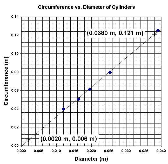
slope = (C2 - C1)/(D2 - D1)
= (0.121 m - 0.006 m)/(0.0380 m - 0.0020 m)
= (0.115 m)/(0.0360 m)
= 3.19 (units divide out)
intercept = -0.001 m
Matching Table
The next step in determining the function that describes the relationship between the variables is to write the equation of the line. In math class, you learned that the equation of a straight line is y = mx + b. You also learned how to determine the values of the slope, m, and intercept, b. In physics class, you have to translate the variables into physically meaningful terms and use corresponding symbols to represent them. You also have to determine values of the slope and intercept and relate these to the physical situation. A matching table provides an aid to writing the equation. The matching table has 6 columns. These are described first.
| Column heading | Meaning |
| Math | standard mathematical symbols |
| maps to | simply indicates a mapping of the generic math variables and constants to the corresponding physical variables and constants for the physical situation under investigation |
| Physics | symbols used to represent the physical variables and constants |
| Value (graph) | values of the slope and intercept as determined using the best-fit line |
| Value (expected) | values of the slope and intercept expected from theory (if known) |
| Units | units of the variables and constants |
The matching table for the experiment at hand is the following.
| Math | maps to | Physics | Value (graph) |
Value (expected) |
Units |
| y | --> | C | m | ||
| m | --> | pi | 3.19 | 3.14 | none |
| x | --> | D | m | ||
| b | --> | none | -0.001 | 0 | m |
Now we can write the equation of the relationship: C = 3.19D - 0.001 m
This is an experimentally-determined relationship between circumference and diameter. However, we also know from theory that C = (pi)D, where pi is 3.14 to 3 significant figures. Therefore, we can say that we expect the slope of the experimental relationship to be pi and the intercept to be 0. In this case, experiment and theory agree on the value of the slope to within 2%. This and the small size of the intercept are easily explained by the errors inherent in the methods of measuring circumference and diameter.
© North Carolina School of Science and Mathematics, All Rights Reserved. These materials may not be reproduced without permission of NCSSM.