Goal

• To investigate the motion of the center-of-mass of a system in a rebounding collision of two objects
• To determine the extent to which momentum and kinetic energy are conserved in the collision

 Introduction

In this lab, you'll investigate a collision of two hockey pucks on a level air table. The pucks each have a magnetic strip, and the two strips repel. Therefore, the pucks don't actually touch. Still, their interaction is a collision, because they exert forces on each other to change the other's velocity. Before continuing, download and view this video clip of a collision.

Since the air table is level and friction is minimal, the system of the two pucks experiences little external force. We would therefore expect that the total momentum of the system is very nearly conserved and that the center-of-mass velocity is nearly constant. If the collision is also elastic, we would expect kinetic energy to be conserved. Kinetic energy is lost in a collision primarily due to the production of thermal energy, sound, and vibration. Such production is greatest for collisions in which one or both objects undergo permanent deformation but is also present for objects that regain their original shapes after rebounding. In the collision of a racquetball with the floor, you saw that the ball changed greatly in shape both during and after the collision. The sound energy produced in a racquetball collision is obvious. The thermal energy is harder to detect, but you would notice a significant warming of the ball after repeated collisions. Therefore, we would expect that there would be significant loss of kinetic energy in racquetball collisions. On the other hand, the collision of hockey pucks is silent and the fact that the pucks don't touch or deform minimizes thermal and vibrational energy loss. There may be some thermal losses, though, from a small amount of friction of the pucks with the table. There could also be gains or losses of kinetic energy due to the fact that the table can't be made perfectly level. Such gains or losses would be due to the external force of gravity. We can determine how much of an effect this has by checking how nearly constant the velocity of a puck is as it slides across the table before or after colliding.

 Data and video analysis

There are several video clips. Select the clip for analysis in the same row with the initial of your last name.

Collision	Last name
ec01	A - D
ec02	E - H
ec03	I - L
ec07	M - P
ec08	Q - U
ec09	V - Z

Overview of the video analysis procedure: Since there are two objects, you'll first mark the positions for one of them, add a point series, and then mark the positions for the other object. You'll scale the video using a marked distance in the video, and you'll position and rotate the coordinate axes conveniently. See the Guide to Using Logger Pro if you need help with software functions.

1. Insert your video clip in Logger Pro and drag the clip to a larger size. The motion starts after the hands have left the pucks and stops before the pucks hit the table bumpers. Therefore, you can mark every frame of the video. Mark as nearly as you can the center point of a puck. Begin with the puck at the top of the screen; we'll call this the upper puck. After marking the frames for that puck, drag the slider back to the start of the clip, add a point series, and mark all the frames for the lower puck. Save your work frequently as you work. The file name is L139-lastnamefirstinitial.cmbl.

2. Set a scale factor using the meter stick near the bottom of the video frame. While the graduations are indistinguishable, the 4 pieces of black tape are positioned 0.100 m apart. That distance is measured from the same side of the tape. Therefore, when you drag the green line across the meter stick to set the scale, you would drag either from the left side of one piece to tape to the left side of another piece or from right side to right side.

3. Do some formatting of the data table before continuing with the analysis. First, delete the 4 velocity columns. Next, rename the position variables. The upper puck is the less massive one; therefore, use the subscript L (for light) to distinguish X- and Y-coordinates. Use H for the lower puck.

4. You may have noticed when you added a point series that there was an option to add a center-of-mass series. You can use that to quickly add columns to your table for the coordinates of the center-of-mass of the two-puck system. Click on the Add Point Series icon and select Add Center of Mass Series. In the Center of Mass dialogue box, enter 0.187 and 0.338 kg for the masses of the pucks. Accept the name for the series and the number of decimal places. When you click OK, the entire point series will be added to the video and the data table. The positions should already be named appropriately in the data table. Don't delete the two new velocity columns this time; if you do, the enter point series will be deleted. (Of course, you can quickly recreate it.) By the way, the reason that we have you delete the velocity columns when possible is that the velocities are calculated using a finite-difference method and therefore show significant variations due to uncertainties in adjacent point placements. A much better way to determine velocities is to fit the position graphs before and after the collision with straight lines and then find the slope. That will come later though.

5. The last thing to do is set the coordinate axes. Drag the origin to a point at about the midpoint of the center of mass series. Then grab the yellow dot and rotate the axes to align with the series. If you want to fine tune the angle of rotation, in the main menu select Insert -> Parameter Control. A window will appear that will allow you to change the angle by 1 degree increments. If you want finer adjustment, in the main menu select Options -> Parameter Control Options. Then change the increment to a smaller value. In order to get rid of the adjustment window so that you don't accidentally change the angle later, thereby shifting all your data, just click on the window and then hit Delete. While it's not essential to positon the axes in this way, it provides some convenience in that the center-of-mass velocity has one negligible component.

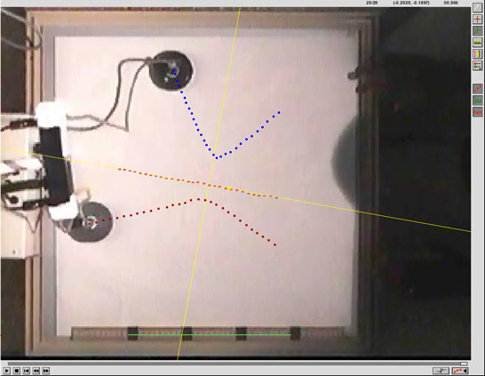
The image to the right shows a completed video analysis. Click on the image for a larger version.

 Analysis and Interpretation

Overview of the graphical analysis procedure: There are 12 velocity components to determine, and each of these are determined by finding the slope of a linear fit of position vs. time. Matching tables and equations of fit aren't required this time. The only information you need to obtain from each fit is the slope. In order to avoid cluttering a single graph with many point series and boxes of fit results, you'll create three graphs, one for each of the pucks and one for the center of mass. You'll find that all this is surprisingly quick to do. Just be careful not to confuse components with each other.

You'll record your results in item 2 of the WebAssign assessment, L139. Open that now.

1. Begin by creating the 3 graphs. Each graph will show plots of X- and Y-positions vs. Time for either one of the pucks or the center of mass. Title each graph to clearly distinguish it from the others: Position vs. Time for the _(insert puck or CM)_ is sufficient. Next you'll determine all the velocity components before and after the collision. When you do this, be sure to avoid the collision region itself where velocities are changing. Click and drag your mouse over the points before or after the collision that appear to be linear and then do a linear fit on each such region. Record your 12 velocity components to 4 decimal digits. Save and submit your Logger Pro file.

2. Enter the following in the table. Enter values to 4 decimal digits. (The momentum and kinetic energy components are checked using your values of the velocity components.)

The masses of the pucks and the mass of the system

The 12 velocity components from your Logger Pro fits

The momentum components, which you will calculate

The initial and final kinetic energies of each puck, which you will also calculate. (Why don't you calculate components of the kinetic energy as you did for momentum?)

Puck or CM	Mass	Velocity Components (m/s)				Momentum Components (kgm/s)				Kinetic Energy (J)
	(kg)	vix	viy	vfx	vfy	pix	piy	pfx	pfy	Ki	Kf
L	<_>	<_>	<_>	<_>	<_>	<_>	<_>	<_>	<_>	<_>	<_>
H	<_>	<_>	<_>	<_>	<_>	<_>	<_>	<_>	<_>	<_>	<_>
CM	<_>	<_>	<_>	<_>	<_>	<_>	<_>	<_>	<_>

Using values in your L and H rows above, calculate the following.

5. The total momentum components for the system of two pucks. Enter values to 4 decimal digits.
6. The total kinetic energies for the system of the two pucks. Enter values to 4 decimal digits.
7. The percentage change in the collision of each of the following: x-component of total momentum, y-component of total momentum, kinetic energy. % Change is calculated using this formula: % Change = 100(Final value - Initial value)/(Initial value). Enter values to 1 decimal digit.

Total Momentum Components (kgm/s)				Total Kinetic Energy (J)		% Change in Total Momentum		% Change in Kinetic Energy
Pix	Piy	Pfx	Pfy	Ki	Kf	Px	Py	K
<_>	<_>	<_>	<_>	<_>	<_>	<_>	<_>	<_>

8. Examine your results for % Change in total momentum. Discuss how nearly momentum was conserved in the collision. Explain the sign of the % Change in terms of external forces that may act on the system. (Note that a large percentage for P_y doesn't necessarily mean a correspondingly large change in that component, since the value of P_y should be nearly 0 if you placed your coordinate axes as instructed.)

9. Examine your result for % Change in Kinetic Energy. Discuss how nearly kinetic energy was conserved in the collision. Explain the sign of the % Change in terms of the conversion of kinetic energy to other forms.

10. Explain in terms of a physics principle why the CM velocity should be constant throughout the collision if the net, external force on the system is 0. Then examine your CM velocity components. The y-components should be nearly 0 due to the way the coordinate axes were set up. What is the % Change in the x-component of the CM velocity.

 Conclusion

Write your conclusion to this lab in item 3 of WebAssign L139.

© North Carolina School of Science and Mathematics, All Rights Reserved. These materials may not be reproduced without permission of NCSSM.