Goal

To measure the acceleration of a glider on an air track using the finite difference method

 Prelab

1. Read the Introduction on this page in order to learn what the finite difference method is and how to use it.

2. Do the WebAssign assessment L109PL. You'll practice using the finite difference method.

 Introduction

How does one measure acceleration in the laboratory?  One way is to use a ticker tape timer. A long strip of paper is taped to an object. As the object moves across a table, for example, the paper is pulled through a device similar to a doorbell ringer, which strikes the tape many times a second. A piece of carbon paper below the tape puts a dot on the tape for each strike. If the object is moving with uniform velocity, the dots are spaced uniformly on the strip as shown below. (Click here for additional information to help with visualing this device. Here's a photo of a ticker tape timer.)

If your task were to measure the velocity of the object, you would do something like this:

1. Lay the strip out on a table with a ruler parallel to the line of dots.
2. Arbitrarily designate the first dot as corresponding to an elapsed time of 0 s.
3. Measure the position of each successive dot on the ruler.
4. Plot a graph of position vs. time.
5. Draw the best straight line through the points on the graph and find its slope.

While a quicker method would have been simply to measure the distance between two adjacent dots and divide by the time interval, that method is less accurate than drawing the graph. Moreover, by drawing the graph, you can verify whether the velocity is constant. If the line bent gradually downward, for example, you might surmise that the object was being slowed by friction.

Now suppose the object is accelerating (speeding up to the right). In that case, the spacing of the dots will increase as shown below.

In order to verify that the acceleration is constant and determine a value for it, you would measure position as a function of time as before. However, a graph of position vs. time would have an increasing slope and, in fact, would be parabolic if the acceleration were uniform. There's a mathematical technique for finding the acceleration from a position vs. time plot. It's called a least-squares quadratic fit. However, we're not ready to do that, since it obscures the physics. The method that you'll use in the present lab will make use of the physics that you know. It's called a finite difference method. It works like this:

Once you have the position vs. time data, select successive pairs of points. Calculate the average velocity, Δx/Δt, for each pair. If the intervals between the points are small enough, the average velocities will be good approximations to instantaneous velocities. Knowing that, plot a graph of the average velocities vs. time. If the acceleration is uniform, then the points should lie in a straight line to within the error inherent in the measurements. The slope of that line is the acceleration.

It actually turns out that when the acceleration is uniform, the average velocity over any time interval is equal to the instantaneous velocity at the midpoint of the time interval. This is only true for uniform acceleration. There will be more about this in the theory section.

Here are the specifics on how to carry out the finite-difference method.

1. Use a data table labeled like the following one but with enough rows for the number of dots.

Index n	Elapsed Time, tn (s)	Position, xn (m)	Change in Position, Δxn (m)	Change in time, Δtn (s)	Average Velocity, Δxn/Δtn (m/s)
0	0
1
2
3

2. The indices are consecutive numbers that mark successive positions of the object starting with the first recorded position. This first position has an index of 0 and an Elapsed Time of 0 s.

3. The Elapsed Time for Index, n, is the total time that passes from t = 0 to the nth position of the object.

4. Position is measured according to whatever ruler scale is used for this.

5. Calculate the Δx's as x_n+1 - x_n-1. That means if you're on row n in the table, you take the value of position for the (n+1) row and subtract from that the position for the (n-1) row. Thus, you associate the difference x_n+1 - x_n-1 with time t_n. (Avoid the temptation to calculate Δx as the difference x_n+1 - x_n. That would mean subtracting the position of one point from the position of the very next point. If you used this method, you wouldn't be able to associate the time with either t_n or t_n+1. There wouldn't be a corresponding row in the table.)

6. Calculating the Δt's is much simpler. This is simply the time difference corresponding to each Δx. That is, Δt is the time it takes to go from position x_n-1 to position x_n+1. These should be the same for every value of n.

7. The Average Velocity for each n is simply the ratio of Δx_n to Δt_n.

8. Once the data table is complete, plot a graph of Average Velocity vs. Elapsed Time. Find the slope of the line to determine the acceleration.

 The Equipment Setup

Rather than using the ticker tape timer described above, the equipment used in this lab will be a glider sliding with very little friction down an inclined air track. A photo of the glider resting on the track is shown below.

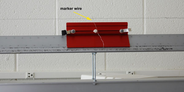
Note the thin wire that is used as a marker. In order to record the motion of the glider, strobe photos were taken of the glider as it slid down the track. The stroboscope flashed at a rate of 10.1 Hz, and recorded a number of overlapping images of the glider on the same frame of film. An example photo is shown below. The glider was sliding from right to left. A very shallow incline was produced by placing a riser block under the right end (not shown) of the track. While the individual images of the glider can't easily be distinguished, the marker wire images can be seen. Click either here or on the photo below to display an enlarged version in a new window. Examine that photo while continuing the reading.

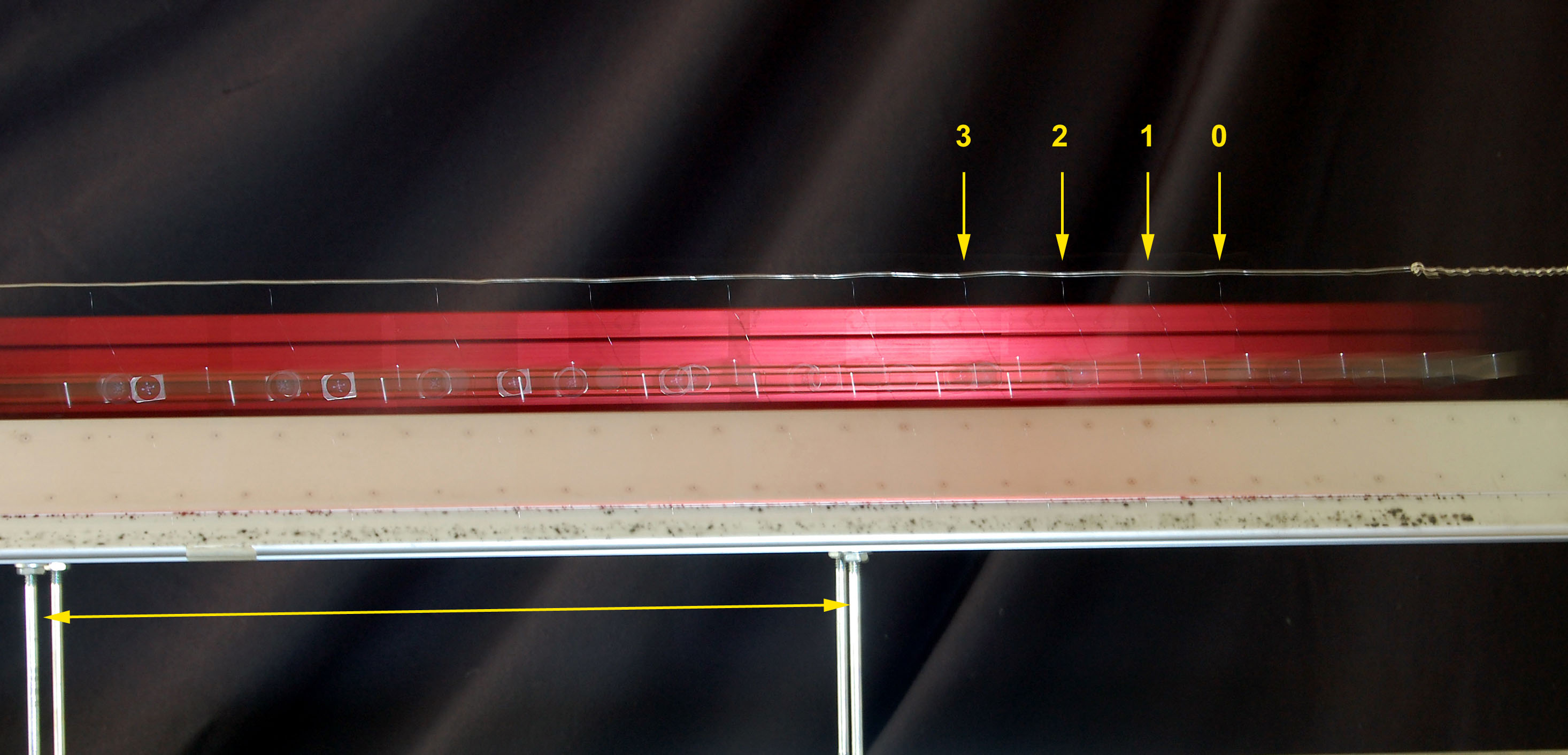
Note the following about the enlarged photo:

• The photo has been annotated to point out the first 4 positions of the wire. Yellow arrows point to these, and the 4 positions are marked 0 to 4.

• While the glider was released from rest, we can't assume that the glider's velocity for the first image was 0. The flash most likely went off a short time after the glider was released.

• The horizontal double-ended arrow below the track indicates the distance between support posts. This is used for scaling distances measured on the photo to actual distances. There are actually 4 support posts shown. They come in pairs, one behind the other. If you viewed a pair of posts head on, you would just see the front post, since the rear post would be hidden behind the front one. The reason you see both posts in a photo is due to optical distortion. This results because the posts are different distances from the camera and are viewed from different angles. To see this for yourself, line up the forefinger of each hand in front of your right eye while keeping your left eye closed. With one finger behind the other, you only see the front finger. Now close your right eye and open your left eye. You'll see both fingers. As you might guess, the presence of this kind of distortion in the photo introduces uncertainty in the calculation of distances.

 Method and Data

1. Print a copy of this table for your data page. This will be your original data page. Follow the usual data-recording procedures. Note that the data table (shown below) has one additional column from the one given in the Introduction. Change in Position has two columns, one for the changes as determined directly from the photo and one for the changes scaled to actual distances.

Image Index n	Elapsed Time tn (s)	Position xn (photo m)	Change in Position Δxn (photo m)	Change in Position Δxn (actual m)	Change in Time Δtn (s)	Average Velocity Δxn/Δtn (m/s)
0
1
2
3

2. Click on the Photo ID below to open in a new window the photo below that corresponds to your position in the alphabet. Print the photo in portrait orientation. The entire photo must print on a single page to be usable, so you may need to set your print options to less than 100% size. Click here for an example of how a photo fits on the printed page. In this case, the print size was 50% of original, but that percentage will depend on your printer. Note that you may print in grayscale as color isn't necessary for the analysis.

Use this photo if your last name begins with...	Photo ID	Riser block height (m)	Frequency of strobe (Hz)
A - E	168	0.0254	10.1
F - J	169	0.0254	10.1
K - O	171	0.0381	10.1
P - R	173	0.0381	10.1
S - Z	175	0.0127	10.1

3. In the Additional Data section of the data page, record the Photo ID, the frequency of the strobe, and the riser block height for your photo. When you record a value, begin with a phrase describing the number that you're going to write, for example, Height of riser block = _________ m.  The phrase tells what the object is as well as what property of the object that you're recording.

4. Three other items of data to record in the Additional Data section are the following.

   1. the actual distance between the air track support posts. This is 0.3050 ± 0.0005 m

   2. the distance between the air track support posts that you measure on your photograph

   3. the scale factor--This is the ratio of item 4a to item 4b

5. Now starting with 0, number the images of the marker wire on your photo consecutively. If your photo has more than 15 marker images, you may stop at 15.

6. Lay a ruler beside the images of the marker wire. There's no need to align the 0 mark of the ruler with spark 0 but you may do so if you wish. Tape the ruler down to the table to keep it from shifting while taking measurements.

7. Read the position of each marker wire image to the nearest 0.0001 m (0.1 mm) using a consistent sighting technique. Record your measurements in the Position column. Record the corresponding Elapsed Time as well. In recording the latter, you'll need to decide how many zeros to place behind the last non-zero number (for example, 0.1 or 0.10 or 0.100). In order to make this decision, use the fact that the stroboscope is accurate and precise to the nearest 0.1 Hz.

8. Calculate the changes in position from the position measurements. Then apply your scale factor to convert the values in photo m to actual m.

9. Complete the Change in Time and Average Velocity columns.

 Submitting your original data page

Scan your original data page and the photo that you analyzed. Save them to a single file that you upload to WebAssign by the date given in the schedule. Name the file L109D-lastnamefirstinitial.pdf. You'll upload your final report at a later date.

 Theory

It's well worth your while to take the time to understand this point, as such an understanding will add a powerful tool to your problem-solving toolkit.

Consider this:

Suppose a uniformly-accelerating object undergoes an increase of velocity, Δv, in a time, Δt. Then in a time Δt/2, which brings one to the middle of the time interval, the velocity will have increased by an amount, Δv/2. In the latter half of the time interval, there is an equal increase of Δv/2 in the velocity. This is the result of uniform acceleration, for which an object undergoes equal increases of velocity in equal times. The average velocity, which is an average over time, must therefore coincide with the middle velocity.

To see that the above is not true for an object with increasing acceleration, let's follow a similar line of reasoning. Over the time interval, Δt, the first increase of Δv/2 in the velocity takes more time than the next increase of Δv/2. That's because the rate at which the velocity increases--that is to say, the acceleration--increases with time. The object spends more time at lower velocities. As a result the average velocity will be less than the middle velocity. It's like the jog-drive problem of P101. In that problem, you jogged and drove the same distance, but you spent much more time jogging than you did driving. As a result, your average velocity for the whole trip was much less than the velocity midway between the jogging and driving velocities.

In the theory section of your report, do the following.

1. Draw a line on a v vs. t graph representing the motion of a uniformly-accelerating object. Make this graph fill half a page for clarity. Next label three widely-separated points on the graph. These points will represent initial and final velocities over a time interval as well as the middle velocity and the time at which it occurs. What it comes down to is that you'll be plotting three points (t_i,v_i ), (t_f,v_f ), and (t_m,v_m ), where i, f, and m represent initial, final, and middle correspondingly. Your graph must make clear the fact that the object increases in velocity from v_i to v_m in the same amount of time as it increases from v_m to v_f..

2. Repeat the previous problem for the case of an object undergoing uniformly-increasing acceleration. (By the way, the actual physics name for the rate of change of acceleration is the jerk. So this will be a case of uniform jerk.) In this case, though, your v vs. t graph must make it clear that the object increases in velocity from v_i to v_m in more time than it takes to increase from v_m to v_f.

3. Now do the following problem. If you apply the key point of this lab, the problem is fairly simple to do. You may find it easier to describe your method in words than to carry out an algebraic solution. Feel free to do so.

   Problem: An object falls from rest without air friction. In the last 0.200 s of its fall, it falls a distance of 20.0 m. What total time was the object falling?

 Analysis

Graphical Analysis

From here on, the analysis will parallel that of L103. In that lab, you drew a graph and best fit line, found the slope, constructed a matching table, and wrote the equation of the fit. You'll carry out these same operations next with your data. You'll draw this graph by hand like you did the one for L103. Here's graph paper if you need it.

1. Prepare your graph paper for a graph of Average Velocity vs. Elapsed Time. If necessary, review the Graphing Guidelines.

2. Draw your best fit line through the data points as best as you can judge it. Select the two points that you'll use to calculate slope.

3. Show the calculation of the slope.

4. Complete the matching table for your line of best fit. This time, we leave you to fill in all the blank cells, except for the Value (expected). We don't expect you know how to determine the latter at this point.

5. Write the equation of your best fit line.

Error Analysis

Complete the uncertainties table to determine the absolute uncertainty in a representative value of the Average Velocity. There are more entries than in L103 due to the fact that the scale factor conversion introduces additional uncertainty. Base your estimate of the absolute uncertainty in the Post separation (photo) on the discussion in the Equipment Setup section. For the elapsed time, information was given in the Method and Data section that should help with your estimate of the absolute uncertainty.

Measurement	Representative Value of Measurement	Absolute Uncertainty	Relative Uncertainty
Position (photo)
Post separation (photo)
Post separation (actual)
Change in time
Average Velocity

1. Explain your estimate of the absolute uncertainty for Post separation (photo).

2. Explain your estimate of the absolute uncertainty for Elapsed Time.

3. Calculate the experimental error in your value of acceleration. Here are the accepted values for the 5 photos.

Photo ID	Accepted value of acceleration (m/s2)
168	0.249
169	0.249
171	0.373
173	0.373
175	0.124

4. Since the measured acceleration depends on Average Velocity and Elapsed Time, assume that the relative uncertainty in the acceleration is the same as that in the Average Velocity. Given that, calculate the absolute uncertainty in the acceleration. Then compare that result to the experimental error. Is your value of uncertainty in the acceleration large enough to account for the experimental error? Tell what you learn by making this comparison.

 Conclusion

State your results to make it clear that you achieved the goal of the lab.

 Review

Before you submit your report, take time to review it to make sure it's complete and properly presented. Once again, here's the rubric.

 Submitting Your Work

Submit the scanned PDF file of your lab report by the due date.

© North Carolina School of Science and Mathematics, All Rights Reserved. These materials may not be reproduced without permission of NCSSM.