You'll give your answers in a WebAssign form. |
Goal
To measure the frequencies of standing waves in open and closed pipes and compare to theoretical predictions
Equipment
You'll need the following items from your lab kit for the prelab.
 LabQuest Mini with USB cable
- Microphone probe
- Toy flute (see photo to right)
- 30-cm ruler
You'll also need a computer for data acquisition.
Prelab
- Read pp. 459-463 of your text.
- View this animation to see the harmonics of an open pipe.
- Follow the instructions in this PowerPoint. Enter your responses in WA L151PL.
Data and Analysis
Preparation: View the video, Harmonics of Open and Closed Pipes, before doing the problems: Streamed / RealPlayer / Flash / MP4
Give your answers to the following in WA L151.
Note about significant figures: Use significant figures correctly throughout this lab. Read scales to the greatest precision possible.
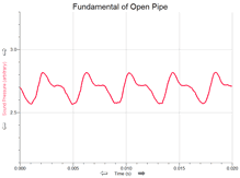
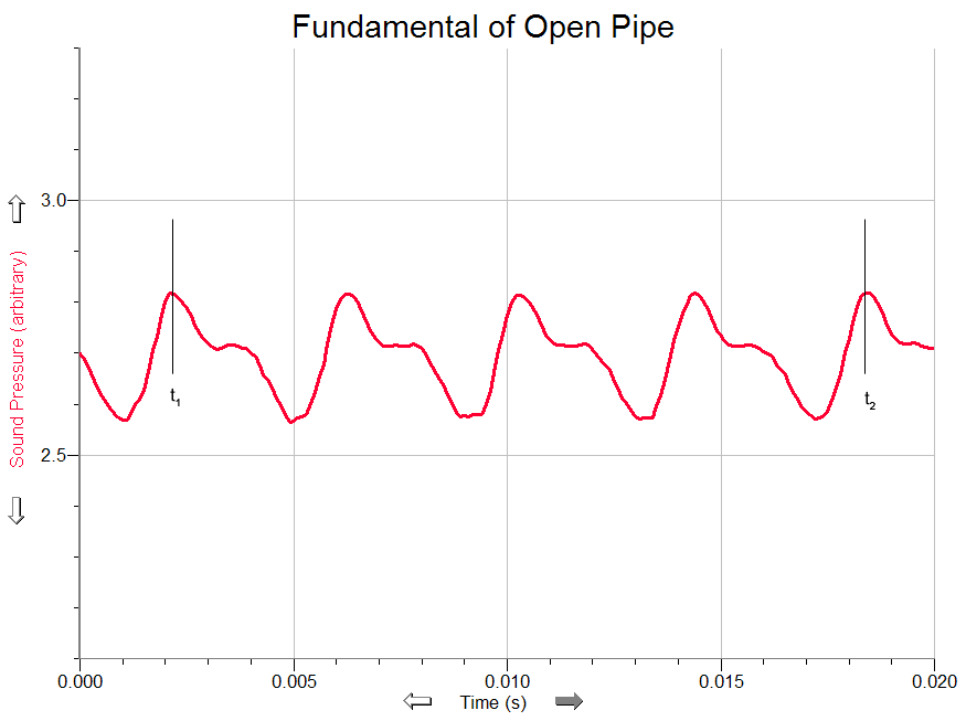
Something the video doesn't show is that a microphone and computer interface were used to collect data on sound pressure vs. time for several of the harmonics. The graph for the fundamental of the open pipe is shown to the right. The waveform isn't a simple sine curve as would be expected for a source of sound producing a tone of a single frequency. That's not unusual. Musical instruments typically produce harmonics of the fundamental at the same time as the fundamental is being sounded. The relative intensities of the harmonics are what give different instruments different sound qualities even when playing the same note. Which harmonic(s) is (are) present for the open pipe, according to the graph to the right? (You should be able to judge this based on work done in L149.)
-
Click on the graph to the right to open a window with an enlarged version. Use the graph to measure the frequency of the sound. If you follow the procedure below, you can expect to determine the frequency to within 2 Hz.
-
Print the graph in landscape orientation. (Remember, larger means a more accurate measurement.)
-
Since the scale divisions aren't marked very fine, here's how you can boost precision. With a ruler, measure the distance to the nearest 0.05 cm on the time axis from 0 to 0.0200 s. (Note that 0.05 cm will correspond to 0.0001 s precision.)
-
Now form a scale factor (SF) between distance and time: SF (cm) = 0.0200 s. Next, measure the distance to the nearest 0.05 cm between the points marked t1 and t2 on the graph.
-
Use your scale factor to convert the distance you just measured to a time.
- Calculate the frequency using f = 4/(t2 - t1). The 4 comes from the number of cycles between the two times. When doing your calculation, don't round intermediate steps. This makes rounding error negligible.
-
-
Now use the method of step 2 to determine the fundamental frequency of the closed pipe. Here's the graph. Note that the time scale is different from the previous graph.
-
Compare your results for the frequencies of the open and closed pipes. Are they what you expect? Explain.