L111. Acceleration of a Falling Object You'll work in a group to develop a theoretical equation to calculate the acceleration of a falling object. Then you'll collect data with the LabQuest Mini interface and calculate the acceleration. You'll compare the result to the accepted value of the acceleration of a freely-falling object near the surface of the Earth.

 Goal

To use the definition of acceleration in a direct measurement of the acceleration due to gravity (to 3 significant figures)

 Introduction

Figure 1

A direct measurement of the acceleration of a falling object requires the measurement of the velocity of the object at two instants of time as well as the measurement of the time interval between these two instants. Let the two velocities be denoted by v_i and v_f and the time interval denoted by Δt = t_f  - t_i. Then the acceleration is given by a = (v_f - v_i)/Δt. Note that in this equation, the velocities are instantaneous velocities.

In practice, v_i and v_f must each be determined by timing the fall of the object through a short distance. Thus, three successive time intervals must be measured in order to determine the acceleration. In this experiment, the task of measuring these 3 intervals is left to a computer triggered by the passage of the object through a photogate. The object is a strip of plexiglass divided into three regions (see Figure 1). Two opaque regions of lengths, d_L and d_U, are separated by a longer transparent region of length, d_C. The strip is held vertically and dropped through the photogate, which consists of a diode which emits infrared radiation and a transistor which detects that radiation. As the strip falls through the photogate, the light path is first blocked by the lower strip L, then unblocked, then blocked by the upper strip U, then unblocked.

The formula a = (v_f - v_i)/Δt uses instantaneous velocities. Experimentally, you'll have to settle for average velocities, since the equipment that you'll be using measures a finite time corresponding to a finite distance of fall. Interestingly, this doesn't introduce error into the experimental determination of acceleration, assuming that the acceleration is uniform. When the latter is the case, the average velocity over a time interval is equal to instantaneous velocity at the midpoint of the time interval. You'll use this fact in the prelab.

Definitions of Symbols

In this experiment, it's important to make a distinction between instants of time and time intervals. First, we define four instants of time. Note that these are points in time as distinguished from time intervals.

Instant of time	Event corresponding to instant of time
t1	lower region of strip breaks photogate beam
t2	lower region of strip leaves photogate beam
t3	upper region of strip breaks photogate beam
t4	upper region of strip leaves photogate beam

Figure 2 below provides a pictorial representation of the positions of the falling strip at the four instants of time. The black rectangle represents the position of the photogate.

Figure 2

With the above notation, the time intervals that will be measured by the computer are the following.

Δt_L = t₂ - t₁ = the interval of time for the lower region of width, d_L, to pass through the gate,
Δt_C  = t₃ - t₂ = the interval of time for the center region of width, d_C, to pass through the gate,
Δt_U = t₄ - t₃ = the interval of time for the upper region of width, d_U, to pass through the gate.

The average velocities of the strip corresponding to time intervals Δt_L and Δt_U will be denoted as v_L,av and v_U,av.

 Theory

Work within your assigned lab group to complete the theory questions below. When you've done so to the satisfaction of the group, you may move on to the Method.

Developing formulas for acceleration and initial velocity

We assume for the following that timing begins at t₁ = 0. Elapsed time is defined as the total time that passes from t₁ = 0.

1. Do the following to develop a formula for the acceleration of the strip.

   1. While v_L,av is an average velocity, the strip has this value of velocity at the midpoint of the time interval during which the lower opaque region is blocking the photogate. That is, the elapsed time t_i at which the strip has instantaneous velocity v_i  = v_L,av is t_i = Δt_L/2. Likewise, there's an elapsed time, t_f, when v_f  = v_U,av. Develop an equation for t_f in terms of Δt_L, Δt_C, and Δt_U only.

   2. Write a formula for Δt = t_f - t_i in terms of Δt_L, Δt_C, and Δt_U only. Express the formula in simplest terms.

   3. Beginning with the definition of acceleration, write a formula for the acceleration a of the strip in terms of these symbols only: d_L, d_U, Δt_L, Δt_C, and Δt_U.

2. When timing begins at t₁ = 0, the stip is already moving. Use the symbol v₁ to represent the velocity of the strip at t₁ = 0. Assume for this problem that the acceleration, a, of the strip is given. The goal is to develop a formula for v₁ in terms of these symbols only: d_L, Δt_L, a. Start with an appropriate dvat.

 Apparatus

From your lab kit:

• LabQuest Mini interface with USB cable
• Vernier photogate with support rod
• Plexiglas strip
• Centimeter ruler

You supply:

• Computer with available USB port
• Cushion (to soften the blow when the strip hits the floor)
• Tape (or other means to anchor the photogate)

 Method

The LabQuest Mini and photogate setup

1. You'll be using the LabQuest Mini interface and Logger Pro for data collection.
2. Connect the LabQuest Mini interface to your computer using the supplied USB cable.
3. Start LoggerPro. The LabQuest interface should be detected automatically. In order to check this, click the icon located in the upper left-hand corner of the Logger Pro window. (See Figure 3 below for the location of the icon.)
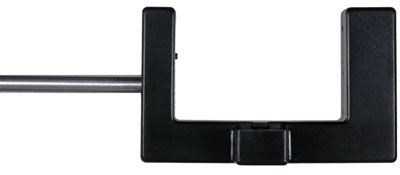
4. Prepare the photogate by screwing the support rod into the photogate as shown in Figure 4.
5. Tape the support rod down to a table or hold it down with a book. The U-shaped gate needs to extend over the table's edge and be oriented horizontally. Figure 5 shows a view of the setup looking down on the table.
6. You'll be dropping the plexiglas strip through the photogate. In order to keep the strip from cracking or chipping when hitting the floor, make sure there's a cushion such as a pillow underneath.

Figure 3	Figure 4	Figure 5

The data collection setup

1. The photogate includes a cable to connect it to the LabQuest Mini. Connect the cable into the DIG 1 port on the Mini. Connect the other end, which is a phone-style plug, to the photogate. Test the photogate by passing your hand through it. A red LED should light on the back of the photogate.
2. In Logger Pro, you'll need to open an experiment file that will collect the data you need. From the Logger Pro menu, make the following selection. Note that the path may a bit different than the one shown. The important thing is to navigate to the Experiments subfolder of the folder where the Logger Pro software is installed on your computer.

• on a Mac: File -> Open -> Applications -> Logger Pro 3 -> Experiments -> Probes & Sensors -> Photogates -> Bounce.cmbl
• on a Windows computer: File -> Open -> Program Files -> Logger Pro 3 -> Experiments -> Probes & Sensors -> Photogates -> Bounce.cmbl

The file that opens says that it's used to determine the coefficient of restitution of a bouncing ball. Don't concern yourself with that. What's important is that the program measures the three time intervals that you need.

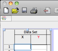
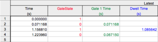
3. You can test the program as follows. At the top click this button, , to start data collection. Hold your fingers together and pass your hand completely through the photogate. Then do it again. The program should have recorded four times and three time intervals. See Figure 6 below for a screen capture of a typical result from Logger Pro. The values listed in the Time column correspond to the times t₁ to t₄ defined previously. Note that the program always sets t₁ = 0. The program gives the time intervals Δt_L and Δt_U in the Gate 1 Time column and the time interval Δt_C in the Dwell Time column. (Ignore the Velocity and Coefficient of Restitution columns.)

Figure 6

4. Assuming everything is working correctly, you can do a test drop. Hold the strip as shown in Figure 7 below. The bottom edge of the strip should initially be above the plane of the photogate. Holding it a few centimeters above the plane of the photogate should be fine for your first drop. Hold the side of the strip vertical and the top of the strip horizontal as nearly as possible. Hold the strip between thumb and forefinger. When you're ready to drop, click the Start Collection button in Logger Pro and pull your fingers apart quickly. Don't record the data yet. Practice dropping until you have a good, repeatable technique. Then move on to the Data section.

Figure 7

 Data

1. Print this form for your data.

2. You'll see that the upper and lower regions of the strip are lettered to avoid confusion. While the widths of these two regions are nearly the same, there may be small differences which can influence the results. With your centimeter ruler, measure the widths of the three regions to a precision of 0.0001 m (that's a tenth of a millimeter). Since the widths of the regions may vary slightly across the strip, measure the widths along the vertical line that will pass through the photogate, as nearly as you can tell. See Figure 8 below.

Figure 8

3. Now you're ready to collect time data. You'll time 4 drops of the strip. For each drop, initially hold the strip so that the bottom edge is a different distance from the plane of the photogate. This means the strip will enter the gate with different initial velocities. The distances to use are already entered into the data table. You need only measure these distances to the nearest centimeter.

 Completing the report

Go to WebAssign L111 to complete the calculations and analysis for the report.

© North Carolina School of Science and Mathematics, All Rights Reserved. These materials may not be reproduced without permission of NCSSM.